Sequence to Sequence Models

输入为一个序列，输出为另一个序列

比如语言翻译

根据图片内容生成对其语言描述

机器翻译过程可以看做是一个有条件的语言模型

找到最合适的翻译结果Y 的过程，就是计算在 x 输入情况下得到Y的概率P，使P达到最大值的过程

相关练习
上述过程更适合直接获取到整个句子Y后，对整个句子的适配度进行概率计算，而不是用贪心算法，
依次根据上一个词的内容找到最匹配的下一个词之后，再最终对整个句子进行概率运算，
因为单个词语查找最合适下一个词语的概率，是计算量非常大的，另外词语的高频性可能会影响句子整体的适配性
比如下面句1 比句2 翻译的效果更好
但是句1和句2 在用贪心算法获取过程中更可能得到句2，因为得到相同的前两个词语之后，going 出现的频率大于visiting

贪心算法的缺点是，在获取到当前词语之后，会根据当前词语，获取下一个词语，然后获取下一个词语，直到获取到整个句子.

集束搜索算法

集束搜索算法（beam search algorithm）: 在获取当前词语之后，会获取当前词语的概率最大的k个词语，然后获取下一个词语，直到获取到整个句子
相当于同时进行集束宽度（eg. B=3）个贪心算法，然后再每一步的n*3 个结果中寻找概率最大前B 个结果，然后进行下一步.n 是当前词汇库中的词汇数
这样就比贪心算法可能得到更多的可能性

优化

当前的概率计算存在以下问题

1. 概率值都是小于1的值，多项相乘时，项数越多，值越小，对于计算来说，能存储的极小值有限，容易出现数据下溢
2. 基于问题1，项越多概率越小，导致模型为使概率值最大，尽可能生成短句子，从而天然倾向生成较短的句子，不倾向生成长句子
3. 对于长句生成本身不友好
   

对于集束宽度的选择
实际生产为10个左右，大于100的基本就可以算做太多了
large B 可以得到更好的结果，但是训练时间会变长
small B 会得到差的结果，但是训练时间会变短

虽然集束搜索算法不如深度或者广度优先搜索算法的准确性高，不能保证找到最准确的值，但是计算速度会比二者快

问题分析

通常增加测试数据集或者增加集束搜索宽度，一般都会是效果更好
但判别是RNN过程有错误，还是集束搜索算法搜索过程有错误可以更根本的解决训练异常问题

如果人工翻译结果概率大于算法得出的句子的概率，即集束算法没有找到使概率最大的正确的句子，问题出在解码查找过程
相反，在本身人工翻译结果好于算法结果的情况下，如果人工翻译结果概率还是小于算法得出的句子的概率，说明RNN过程有错误

bleu 算法

类似图像识别可以用对错一个确定的数值判断推测结果，这里用bleu 算法得到的指数来评估翻译结果好坏
用来计算评估机器翻译结果的指数，从而评估翻译好坏
翻译越接近人类翻译，指数分数越高
具备双语评估，且具有人类评估结果替补性

短翻译容易获得高精度的评判结果，为了降低这种误差，引入BP 惩罚参数进行更精准效果计算

注意力机制

之前涉及的机器翻译是使用两个rnn 结构，先编码后解码（编码后将信息存在激活函数中），一次性读取整个句子会之后再整体翻译
这样对于特别长的句子来说不太现实，即需要处理的入参特别长，随着句子长度增加，bleu 指数会有明显下降
且不符合人类翻译习惯，人类翻译更倾向于，读一段翻译一段，这样只关注一整段文字里面的一小段句子

注意力机制在编码阶段会生成一系列输入单词的特征信息（单词本身和它周围词的特征），
在生成翻译结果时，根据输入句子中每个单词对该翻译结果单词的影响权重（注意力权重）和已经翻译出的单词两个信息共同计算出当前单词的翻译结果

具体计算过程


更多应用，日期格式转换

应用

语音识别，输入变成每一帧的语音音频, 1秒有1000帧的话，输入就会是1000个数据，相当于上面1000个单词


触发词识别

transformer

对于循环神经网络来说，rnn, Lstm 处理连续输入信息会要求神经网络越来越复杂

将注意力机制中RNN 过程用CNN 卷积 同时处理多个单词的过程就是transformer 架构

transformer 架构的模型两个关键点

1. 自注意力机制 — 带着句子上下文情况下特征计算
2. 多头注意机制 — 自注意力机制循环过程，产生多种可能性

自注意力机制

计算输入单词的注意力值

多头注意力机制

在自注意力机制基础上，同时并计算其他多个问题的注意力值
通过并行同时获取多个单词之间的不同维度的含义关系

transform 网络

有时候使用mask multi-head attention 进行训练
在有准确输入输出情况下，
在解码阶段，将输入值从正确输出结果里一次掩盖后几个单词，假设还没有推理出来，仅推理出了前几个单词
查看能否正确预测出序列中的下一个单词

word representation 词汇表征

如果用one-hot表示词汇集中的word，只能存储这个单词在这个词表中的索引，无法表示单词的语义，更无法计算不同单词之间的相似度/关联度。
如果选取n个features, 每个feature 再用数据大小表征当前单词和这个feature的关联度，可以更好的表征单词语义和计算单词之间的相似度，从而进行词嵌入，进一步进行猜词计算

引入坐标系的概念，如果n个特征代表n 个维度,比如300个维度，那么每个单词就像嵌入在这个300维空间中, 会自然的发现类似的或者同类的单词会聚集在一起
使用t-sne 算法通过降维到2维可以实现词分布的可视化

词嵌入应用

实体识别 ==> 迁移学习

因为现在每个单词是通过词嵌入表征的，所以如果对于已经识别的实体，对于现在要识别的实体，只需要对比特征向量的相似度，就可以进行识别
另外，对于词汇表中未出现的单词，通过进行特征向量转换后，自然可以加入词汇表中，从而可以直接进行相似度计算

词嵌入方便进行迁移学习，尤其是大批量词嵌入模型应用与小批量垂类领域时，需要重新进行词嵌入的新词是少数，可以直接使用词嵌入模型中已存在的大多数语义逻辑，从而进行迁移学习

词嵌入迁移过程

词嵌入word embedding 和 之前的人脸识别的 face encoding 思路一致，可以认为是意思一样的术语

更多： 文本摘要（text summarization）文本解析（co-reference resolution）解析（ parsing）

类比推理

使用余弦相似度算法或者其他可以计算相似度的算法，可以对两个已知单词进行向量计算，得到向量关系，从而推理出问题中单词在相同向量，即类比关系中对应的单词

比如 Q: man 对应 woman 那么 king 对应 ?
a: eman - e_woman = e_king - e?

e? = e_king - e_man + e_woman
如果向量 e? 和 e_king - e_man + e_woman 相似度值越高，即词语语义越相似，越接近正确答案

使用余弦计算相似度
两个向量夹角角度的余弦值，夹角为90度时，余弦值为0, 夹角为0度时，余弦值为1， 夹角为180度时，余弦值为-1，相反方向

词嵌入矩阵

所有词汇表中的单词进行特征向量表示后，组成的矩阵，如果跟原来one-shot表示法中某个单词w的向量进行点积运算可以直接得到该单词w 的特征向量表示
E · O_w = e_w

使用word embedding 进行模型训练

整体步骤都是将样本数据（一个句子）中单词分为目标值和输入值后，形成监督学习模型，然后进行训练

1. 将目标值转成特征向量，摊平所有的向量值
2. 引入softmax 激活函数，计算目标值出现的概率，取概率最大的值与目标值对比
3. 计算损失函数，重新训练

词嵌入矩阵的训练过程

优化

1. 固定输入单词数量，如上例，输入值为推测词前面的所有6个单词，300维的特征摊平后，输入值为300 * 6 = 1800维
   如果固定单词数量为4，输入单词数量减少，那么特征向量的维度也会减少，模型输入值减少，从而可以减少训练时间
   固定输入单词数着窗口，可以方便的处理任意长度的句子，因为这样模型的输入结构就是固定的

2. 尝试使用不同的上下文选取窗口大小进行训练
   最近4个
   左右各4个
   最近1个
   附件的一个

3. 使用 Word2Vec 中的 Skip-grams 算法进行训练
   Skip-grams 先固定输入上下文，在根据不同窗口规则选取目标值，生成监督学习数据对

softmax 分类 的问题就是要全量计算所有的概率，然后取概率最大的值，这样计算量非常大

4. 负采样
   选取一对正确的目标值和上下文，作为输入， 输出为正确的flag 1， 作为正采样样本
   然后随机生成k个负采样样本，负采样样本输入值中的上下文和正采样样本一致， 目标值随机选取，输出为错误的flage 0

   
   正采样样本和负采样样本一起组成监督学习样本对 进行训练
   这样做的好处，相当于原来要判断单词集合中所有单词是不是正确答案，错误答案是远多于正确答案的，现在只要判断k个单词生成的错误答案，避免了每次判断所有的单词，从而大大减少计算量
   
   负采样单词的获取为了避免取到极高频词或者极低频词，一般用下面的概率公式判断当前单词概率，决定是否要采样，f(w) 为单词出现频率
   

5. 情感分类
   将评论中单词进行特征向量转换后进行均值计算，最后对计算结果进行softmax 分类
   
   但这样没有考虑单词之间的语序和重复出现的频率问题，会导致预测结果不准确
   可以使用RNN 进行训练, 解决单词语序引起的语义失真问题
   

   相关练习

6. 语义纠偏
   

相关练习

文生视频

1. 找到相似图片，通过文心一言生成图片提示词
2. 将提示词替换下面代码, 在jupyter notebook中运行可以得到5张图片

1
2
3
4
5
6
7
8
9
10
11
12
13
14
15
16
17
18
19
20
21
22
23
24
25
26
27
28
29
30
31
32
33
34
35
36
37
38
39
40
41
42
43
44
45

import json
import os
import dashscope
from dashscope import MultiModalConversation

# 以下为北京地域url，若使用新加坡地域的模型，需将url替换为：https://dashscope-intl.aliyuncs.com/api/v1
dashscope.base_http_api_url = 'https://dashscope.aliyuncs.com/api/v1'

messages = [
    {
        "role": "user",
        "content": [
            {"text": "一张充满秋日氛围的摄影图，画面中心是一片金黄的枫叶，叶脉清晰、边缘略带枯黄斑点，阳光从画面右侧洒下，形成耀眼的光斑与柔和的光线；背景是暖色调的树木（树叶呈橙红渐变），远处有朦胧的建筑轮廓；整体风格自然写实，光线明亮且带暖调，营造出宁静又诗意的秋日氛围，细节上突出枫叶的质感与光影层次。"}
        ]
    }
]

# 若没有配置环境变量，请用百炼API Key将下行替换为：api_key="sk-xxx"
# 新加坡和北京地域的API Key不同。获取API Key：https://help.aliyun.com/zh/model-studio/get-api-key
api_key = "xxxxx"
for  i in range(0,5):
    response = MultiModalConversation.call(
        api_key=api_key,
        model="qwen-image-plus",
        messages=messages,
        result_format='message',
        stream=False,
        watermark=True,
        prompt_extend=True,
        negative_prompt='',
        size='1328*1328'
    )
    
    if response.status_code == 200:
        print(json.dumps(response, ensure_ascii=False))
        import requests
        url = json.dumps(response, ensure_ascii=False)
        reponse = requests.get(url=response.output.choices[0].message.content[0]['image'])
        with open('./ad50000'+str(i)+'.png','wb') as f:
            f.write(reponse.content)
    else:
        print(f"HTTP返回码：{response.status_code}")
        print(f"错误码：{response.code}")
        print(f"错误信息：{response.message}")
        print("请参考文档：https://help.aliyun.com/zh/model-studio/developer-reference/error-code")

3. 将图片上传到度加-视频生成，生成依据图片生成的视频

商品评论分析

1
2
3
4
5
6
7
8
9
10
11
12
13
14
15
16
17
18
19
20
21
22
23
24
25
26
27
28
29
30
31
32
33
34
35
36
37
38
39
40
41
42
43
44
45
46
47
48
49
50
51
52
53
54
55
56
57
58
59
60
61
62
63
64
65
66
67
68
69
70
71
72
73
74
75
76
77
78
79
80
81
82
83
84
85
86
87
88
89
90
91
92
93
94
95
96
97
98
99
100
101
102
103
104
105
106

# Python3.8以上
pip install pydantic==2.5.3 -i https://mirrors.aliyun.com/pypi/simple/
pip install  langchain-core==0.1.45 -i https://mirrors.aliyun.com/pypi/simple/
pip install langchain==0.1.16 -i https://mirrors.aliyun.com/pypi/simple/
pip install  dashscope==1.24.7 -i https://mirrors.aliyun.com/pypi/simple/

#导入库
import os
import pandas as pd
from typing import List, Optional
from langchain_core.pydantic_v1 import BaseModel, Field
from langchain_core.utils.function_calling import convert_to_openai_tool
from dashscope import Generation
import dashscope
from langchain.tools.render import render_text_description
import warnings
warnings.filterwarnings('ignore')

# 1.初始化大模型环境

# 使用大模型类型
os.environ["DASHSCOPE_API_KEY"] = "https://dashscope.aliyuncs.com/compatible-mode/v1"

dashscope.api_key = "xxx" // 阿里云百炼 https://bailian.console.aliyun.com/?tab=model#/api-key

from typing import Optional

from langchain_core.pydantic_v1 import BaseModel, Field


class Person(BaseModel):
    """Information about a person."""
    name: Optional[str] = Field(default=None, description="The name of the person")
    hair_color: Optional[str] = Field(default=None, description="The color of the peron's hair if known")
    height_in_meters: Optional[str] = Field(default=None, description="Height measured in meters")

2.读取数据

df=pd.read_excel(r"./原始数据.xlsx")

df.head(2)
df[df["Rating"]<2].groupby("Clothing_ID").size().sort_values().tail(10) # 评分低于2的最多的10条数据

3.筛选数据
re_862=df[(df["Rating"]<2)&(df["Clothing_ID"]==862)].Review_Text.dropna(axis=0,how=any).tolist() // 去掉Review_Text 缺省的数据

4.大模型处理

# 定义问题类别
class clothing(BaseModel):
    Fabric_problems: Optional[str] = Field(default=None, description="Fabric problems: noticeable holes, loose threads, pilling, or abnormal color fading and shrinkage")
    Workmanship_defects: Optional[str] = Field(default=None, description="Workmanship defects: poor stitching, excessive loose threads, easily detachable buttons, etc")
    Size_discrepancies : Optional[str] = Field(default=None, description="Size discrepancies: the actual product size differs from the described dimensions, leading to ill-fitting garments.")
    Uncomfortable_wear : Optional[str] = Field(default=None, description="non-breathable fabrics, irritation against the skin, or discomfort during wear.")
    Fit_design: Optional[str] = Field(default=None, description="Fit and design: unsuitable cut, not conforming to ergonomics, or unflattering when worn")
    Appearance_Discrepancies: Optional[str] = Field(default=None, description="Mismatch between the product received and online images in terms of style or color.")
    After_Sales: Optional[str] = Field(default=None, description="Unsatisfactory customer service attitude or response efficiency.")
    Value_Money: Optional[str] = Field(default=None, description="Consumers feel that the price does not align with the actual quality or value of the product, perceiving it as overpriced.")

class Data_yun(BaseModel):
    """提取负面信息"""
    comment: List[clothing]

# 封装请求数据
def prompt_yun(ct):
    system_prompt="您是提取算法专家。仅从文本中提取相关信息。如果您不知道要求提取的属性值，则为属性值返回 null。首先抽取出用户评价中的抱怨点，然后对这些点进行分类，然后调用工具输出"
    prompt=[{"content":system_prompt,"role":"system"},\
            {"role":"user","content":"The material is cheap"},\
            {'role': 'assistant', 'content': '', 'tool_calls_ids': [{'function': {'name': 'Data_yun', 'arguments': 
                                                                              '{"comment": [{"Fabric_problems": "The material is cheap","Size_discrepancies": "is made for women with long torso and shorter shoulders"}]}'}}]}]
    prompt.append({"role":"user","content":ct})
    return prompt

# 向大模型提问
def get_response_1t(mess):
    response = Generation.call(
        model='qwen-plus',
        messages=mess,
        tools=[convert_to_openai_tool(Data_yun)],
        result_format='message', # 将输出设置为message形式
    )
    return response

5.处理单个评论，进行模型能力测试

text = re_862[1]
p_y = prompt_yun(text)
res = get_response_1t(p_y)

res.output.choices[0].message["tool_calls"][0]['function']['arguments']


6.循环处理所有数据

import time
import numpy as np
for i in re_862:
    time.sleep(0)
    text = i
    if text is np.nan:
        print("数据为空值")
    else:
        p_y=prompt_yun(text)
        res=get_response_1t(p_y)
        print(res.output.choices[0].message["tool_calls"][0]['function']['arguments'])
        print('-'*20)

推荐算法1

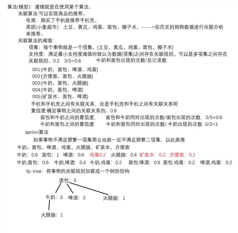
算法(模型): 建模就是在使用某个算法。

关联算法: 可以实现商品的推荐。

电商: 购买了手机就推荐手机壳。

美团(小象超市): 土豆、黄瓜、鸡蛋、面包、椰子水。—>你历史的购物数据进行关联分析来推荐。

关联算法的阈值:

项集: 每个事物就是一个项集。(土豆、黄瓜、鸡蛋、面包、椰子水)

支持度: 满足最小支持度阈值时就认为数据(项集)之间存在关联规则。可以是多项集之间存在关联规则。0.2 3/5=0.6 牛奶和面包出现的次数/总记录数

001:(牛奶、面包、啤酒、鸡蛋)
002:(方便面、面包、火腿肠)
003:(牛奶、面包、火腿肠)
004:(牛奶、面包、啤酒)
005:(矿泉水、面包、啤酒)

手机和手机壳之间有关联系，还是手机壳和手机之间有关联系呢

置信度: 确定事物之间的关联关系的。0.8
面包和牛奶之间的置信度: 面包和牛奶同时出现的次数/面包出现的次数, 3/5=0.6
牛奶和面包之间的置信度: 牛奶和面包同时出现的次数/牛奶出现的次数 3/3=1

apriori算法
如果事物不满足频繁一项集那么也就一定不满足频繁二项集，以此类推

牛奶、面包、啤酒、鸡蛋、火腿肠、矿泉水、方便面

牛奶: 0.6 面包: 1 啤酒: 0.6 鸡蛋0.2 火腿肠: 0.4 矿泉水: 0.2 方便面: 0.2

牛奶: 面包: 0.6 牛奶: 啤酒: 0.4 牛奶: 鸡蛋: 0.2 面包: 啤酒: 0.6 面包: 鸡蛋: 0.2 啤酒: 鸡蛋: 0.2

fp-tree: 将事物的关联规则加载成一个树形结构

面包: 5

牛奶: 3 啤酒: 3 火腿肠: 1

火腿肠: 1

1
2
3
4
5
6
7
8
9
10
11
12
13
14
15
16
17
18
19
20
21
22
23
24
25
26
27
28
29
30
31
32
33
34
35
36
37
38
39
40
41
42
43
44
45
46

import pandas as pd
import warnings
warnings.filterwarnings("ignore")

1.读取数据

df = pd.read_csv('./fruit_purchases1.csv',sep=';')
df.head()

2.数据预处理

df_mtix = df['购买水果'].map(lambda line:line.replace(' ','').split(','))
或者
list_all_f  = []
for x in df['购买水果']：
 list_all_f.append(x.split(','))

from mlxtend.preprocessing import TransactionEncoder

model_te = TransactionEncoder()  # 设置参数
df_te = model_te.fit_transform(df_mtix)  # 应用到数据上
df_te = pd.DataFrame(data=df_te,columns=model_te.columns_)  # 转型

3.关联规则建模
from mlxtend.frequent_patterns import fpmax,fpgrowth,apriori // 不同的计算置信度的算法

model_apriori = apriori(df=df_te,min_support=0.2,use_colnames=True)
# model_fpmax = fpmax(df=df_te,min_support=0.1,use_colnames=True)
# model_fpgrowth = fpgrowth(df=df_te,min_support=0.1,use_colnames=True)

4.association_rules 函数来找出关联规则
from mlxtend.frequent_patterns import association_rules

rules = association_rules(df=model_apriori,metric='confidence',min_threshold=0.8)
rules

5. 推荐---当用户购买了某个水果后应推荐什么其他的水果

buyfruit = input('现已经买了什么水果')

lists = rules[rules['antecedents'] == {buyfruit}]['consequents'].values
print('用户购买了'+ buyfruit + '推荐', lists)

后续策略
去重
如果是一个任何关联都没有的水果，可以推荐support 最高的，购买次数最多的项集

推荐算法2

1
2
3
4
5
6
7
8
9
10
11
12
13
14
15
16
17
18
19
20
21
22
23
24
25
26
27
28
29
30
31
32
33
34
35
36
37
38
39
40
41
42
43
44
45
46
47
48
49
50
51
52
53
54
55
56
57
58
59
60
61
62
63
64
65
66
67
68
69
70
71
72
73
74
75
76
77
78
79
80
81
82
83
84
85
86
87
88
89
90
91

<!-- 想要向某个用户去推荐音乐：
    计算处用户和哪些用户相似，在将和用户相似的用户听过的音乐，并且是用户没用听过的音乐，推荐给用户。
    张三：李四、王五   音乐：1 2 3 4 5 6
    李四：音乐：1  5  6  7  8 
    王五：音乐：2  4  7  9
    向张三推荐：7  8  9
1.计算用户之间的相似度：
2.相似的用户听过的音乐；
3.相似用户听过的音乐哪些是用户没有听过的的；
4.推荐 -->

# 导入pandas和numpy库
import pandas as pd
import numpy as np
# 读取数据集
user_artists = pd.read_csv('./music/user_artists.dat', sep='\t') # 优用"t'分隔符读取user artists.dat文件
artists = pd.read_csv('./music/artists.dat', sep='\t', usecols=['id', 'name']) # 使用t分隔符读取artists.dat文件，仅读取id和name列
user_artists

# 去除不必要的列
# user_artists = user_artists.drop(['weight'], axis=1)# 删除user _artists中的weight列

artists.head()

artists['id'] =artists['id'].astype(np.int64)

6.将user_artists和artists两个DataFrame进行合并，以user_artists中的artistID和artists中的id为键值进行连接。
# 合并数据集
data = pd.merge(user_artists, artists, left_on='artistID', right_on='id') # 将user_artists 和 artists 合并
data = data.drop(['id', 'artistID'], axis=1) # 删除data 中的id 和artistID 列
data

7.去除评分次数少于50次的音乐和用户。
counts = data['userID'].value_counts() # 计算每个用户的评分次数
data = data[data['userID'].isin(counts[counts >= 50].index)] # 去除评分次数少于50 次的用户

counts = data['name'].value_counts() # 计算每个音乐的评分次数
data = data[data['name'].isin(counts[counts >= 50].index)] # 去除评分次数少于50 次的音乐

# 将音乐和用户ID 转换为数字
name_to_index = {} # 创建 name_to_index 字典
index_to_name = {} # 创建index_to_name 字典
for i, name in enumerate(data['name'].unique()): # 遍历 data 中的name 列
    name_to_index[name] = i # 将name 映射到数字
    index_to_name[i] = name # 将数字映射到name
    
user_id_to_index = {} # 创建user_id_to_index 字典
index_to_user_id = {} # 创建index_to_user_id 字典
for i, user_id in enumerate(data['userID'].unique()): # 遍历data 中的userID 列
    user_id_to_index[user_id] = i # 将user_id 映射到数字
    index_to_user_id[i] = user_id # 将数字映射到user_id
data['name_index'] = data['name'].apply(lambda x: name_to_index[x]) # 将data 中的 name 映射到数字
data['user_index'] = data['userID'].apply(lambda x: user_id_to_index[x]) # 将data 中的 user_id 映射到数字
# # 构建用户-音乐评分矩阵
n_users = len(user_id_to_index) # 获取用户数量
n_artists = len(name_to_index) # 获取音乐数量
ratings_matrix = np.zeros((n_users, n_artists)) # 创建用户-音乐评分矩阵
ratings_matrix

8.将data中的评分填入用户-音乐评分矩阵，使得ratingsmatrix的输出为。
for row in data.itertuples(): # 遍历data
    ratings_matrix[row[5], row[4]] = row[2] # 将data 中的评分填入用户-音乐评分矩阵
    print(row)
ratings_matrix
#     print(row)
# 计算用户之间的相似度
from sklearn.metrics.pairwise import cosine_similarity # 导入sklearn 库中的余弦相似度计算函数
user_similarity = cosine_similarity(ratings_matrix) # 计算用户之间的相似度
# 为用户推荐音乐
user_index = 0 # 设置用户索引


9.获取与用户最相似的用户索引similar users(不包括自己)，使得similar users的输出为:
similar_users = np.argsort(-user_similarity[user_index])[1:] # 获取与用户索引为0 的用户最相似的用户索引
similar_users  
recommended_artists=[]# 创建推荐音乐列表

10.填补以下程序，获取相似用户评分的音乐索引artists_rated。

for i in similar_users: # 遍历相似用户索引
    artists_rated = np.where(ratings_matrix[i] > 0)[0] # 获取相似用户评分的音乐索引
    for j in artists_rated: # 遍历音乐索引
        if ratings_matrix[user_index][j] == 0: #用户未评分
            recommended_artists.append((j, ratings_matrix[i][j])) # 将音乐加入推荐音乐列表
recommended_artists = sorted(recommended_artists, key=lambda x: x[1], reverse=True)[:10] # 筛选出推荐音乐中的前10 首
for artist in recommended_artists: # 遍历推荐音乐
#     print(artists[artists['name'] == index_to_name[artist[0]]]['name'].values[0]) # 打印推荐音乐
    print(index_to_name.get(artist[0]))
#     print(artist)

artists[artists['name'] == index_to_name[artist[0]]]['name'].values[0]

实验

csv 文本文件，没有多余格式，适用于各种场景使用，不仅适用各种算法，也适用数仓

jupyter notebook
执行: shift + 回车
注释：control + / ===>解释性文字
收起执行的结果： 点击蓝色边框

python install pandas numpy
pandas numpy 数据分析，数据挖掘

建模

拆分数据：

纵向拆分
x: 除目标列以外的列
y: 目标列

横向拆分：
训练集：模型学习
测试集： 验证模型效果

特征处理

特征缩放
数值类型的数据取值范围差异较大，导致模型在建模的时候忽略了某些属性对模型的重要度，
所以就需要通过特征缩放来平衡属性之间的权重

方法：标准化，最小值，最大值归一化

特征离散化
离散化：将连续数据转换成离散数据
数值的属性范围较大导致模型进行判断条件变多，进而影响模型效率
方法：
分箱： 1,1,1,1,1,1,4,5,1,10
等宽分箱：每个区间的范围大小是相同的
0-5 6-10
[1,1,1,1,1,1,4,5] [10]
等频分箱：每个区间的样本数量相同
[1,1,1,1,1] [1,1,4,5,10]

基于聚类的离散化
基于信息熵的；离散化
基于卡方的离散化
1R

特征编码
有一些模型无法处理字符串类型的数据，这个时候就需要通过特征编码将字符串类型数据转换成模型可以处理的数据

方法：

label-encoding(标签编码)： 将字符串映射为对应数字eg: male –> 0, female –> 1，应用于二元属性和序数属性
one-hot-encoding(独热编码)： 将字符串转换为不同的01组合，应用于标称属性（没有大小顺利的特征）

代码的方式

1. 读取文件

1
2
3
4
5
6

pip install pandas
pip install numpy


df = pd.read_csv('./wine3.csv')
df.head()

2. 缺失值处理方式

删除：

按行删除：

按列删除： 该列数据超过20%缺失，可以考虑删除该列

填充： 通过特殊值填充，如：均值（数据为浮点性），中位数，众数（数据字符串），0

sklearn 也可以处理缺失值，填充 算法预测

1
2
3
4
5
6
7
8
9
10
11
12
13
14
15
16
17
18
19
20
21
22

df.isnull().sum()

df.shape # 查看行列数

del df['phenols'] # 删除列

df.shape

df.info() # 查看每列数据类型

<!-- np.nan 代表缺失值，可能是上面提到的三种 -->

# 填充
df['malic'] = df['malic'].replace(np.nan,df['malic'].mean()) 

# aixs : 0 按行删除； 
# how :any 只要有一个数据缺失就将该行删除，all 表示这一行全部缺失的时候才删除

df_drop = df.dropna(axis= 0, how='any') 

df_drop.isnull().sum()

3. 异常值处理

异常值：

偏离正常样本过多的值，也叫噪声点，离群点，一般是极大或者极小的值

但不是错误值，只有数值类型（有数值含义）数据才会有异常值

处理：同缺失值
删除： 按行删除
替换： 使用特殊值替换，（当做缺失值处理）

异常值检测

箱线图
Q3 + 1.5IQR < X < Q1 - 1.5IQR
IQR = Q3 - Q1
Q3: 75% 分位数 Q: 25% 分位数
1.5 : 经验值，可容忍范围，可根据实际情况调整

3σ 原则: z-score
|x- μ| > 3σ
σ 标准差 μ 均值

务必根据实际情况分析， 比如年龄,可以设定 1-100 范围为正常值，则不需要再进行上述检测

1
2
3

import matplotlib.pyplot as plt
plt.boxplot(df_drop['malic'])
plt.show()

3.1 箱线图：进行异常值检测

1
2
3
4
5
6
7
8
9
10
11
12
13
14
15
16
17
18
19
20
21
22

while True:
    list_error = []
    Q1 = df_drop['malic'].quantile(0.25)
    Q3 = df_drop['malic'].quantile(0.75)
    IQR = Q3 - Q1
    up = Q3 + 1.5*IQR
    down = Q1 - 1.5*IQR
    n = 0
    for x in df_drop['malic']:
        if x > up or x<down :
            print(x)
            df_drop.loc[:, 'malic'] = df_drop['malic'].replace(x,df_drop['malic'].mean()) # 填充 
            list_error.append(x)
    if len(list_error) == 0:
        break


for x in df_drop['malic']:
    if x > up or x<down :
        print(x)
plt.boxplot(df_drop['malic'])
plt.show()

3.2 3σ 原则: z-score
|x- μ| > 3σ

1
2
3
4
5
6
7
8
9
10

mport  warnings
warnings.filterwarnings('ignore')

mean = df_drop['ash'].mean()
std = np.std(df_drop['ash'])
for x in df_drop['ash'].index:
    if np.abs(df_drop['ash'][x] - mean)>3*std:
        print(df_drop['ash'][x])
        df_drop.drop(axis=0,index=x,inplace=True)

4. 拆分数据

1
2
3
4
5
6
7
8
9

# 纵向拆分
X= df_drop.drop(axis=1, columns='type')
Y = df_drop[['type']]

pip install scikit-learn

from sklearn.model_selection import train_test_split

X_train,X_test,Y_train,Y_test = train_test_split(X,Y,test_size=0.3)

5. 建模

1
2
3
4

from sklearn.neighbors import KNeighborsClassifier

model_knn = KNeighborsClassifier()
model_knn.fit(X_train, Y_train)

6. 评估

1

model_knn.score(X_test,Y_test)

7. 保存模型

1
2
3
4
5

pip install joblib

import joblib

joblib.dump(model_knn, './红酒等级预测.pkl')

8 预测

1
2
3

import pandas as pd
import joblib

8.1 读取数据

1
2

df = pd.read_csv('./wine3_pre.csv')
df.head()

8.2. 读取模型

1

model = joblib.load('./红酒等级预测.pkl')

8.3. 预测数据

1
2
3
4
5
6

<!-- 把要预测的数据处理成跟训练的时候的维度一样 -->
del df['phenols']
model.predict(df)

Y_pre = model.predict(df) # 预测
df['type'] = Y_pre # 合并数据

8.4 存储预测数据

1

df.to_csv('./wine_model_pre.csv', index=False)

在线练习

使用 knime

软件下载，要翻墙 https://www.knime.com/downloads

1. 创建工作流
   

2. 添加数据源
   将csv Reader 拖到工作流绘制中心，并只指定训练数据文件
   
   切换 transformation tab 可以指定要保留的列数据，和修改该列数据类型
   

也可以再后续添加 string Replacer 进行具体数值转换

看起来一次只能改一个值，多个值进行转换，可以添加多个string Replacer

3. 缺失异常值处理

添加misssing Value, 对常见数据类型添加缺失值处理规则

也可以对指定列进行缺失值处理规则指定

4. 训练模型
   选择算法指定，目标列
   注意knime 只允许 数据类型为string 的列作为目标列，不是的话，要在前面步骤中进行转换
   

5. 模型预测和结果保存
   注意训练模型的算法和预测的算法要一致
   添加模型预测，结果保存,csv Writer 需要指定保存的文件路径名称
   

业务场景分类

文本处理：LLM（自然语言处理）

视频图片：计算机视觉

混合模型：文本、图片、视频、音频。

任务类型

训练任务：通常是数据量较大，导致计算量也比较大。并行度也高。对资源消耗比较大。对时效性没有太大要求。
推理任务：是使用已有大模型对现有情况处理，数据量通常不大，所以资源消耗没那么大。通常要求处理速度快。

硬件选择

服务器：要评估业务的资源使用情况来具体配置
国产化GPU：昇腾
国产化CPU：华为、海光
操作系统：Linux、欧拉、麒麟

还要考虑以上4者之间的兼容性。

计算资源

全部使用GPU： 耗费高，适用于中大型企业，
GPU+CPU的组合：适用于 中小企业部署，如果用CPU 替换GPU, 所用CPU 数量将是原理GPU 数量的两倍。

华为云 - 工作台 - AI NOTEBOOK 支持使用NPU 进行训练

阿里云 - MODEScope - My Notebook 支持使用GPU

模型选择/模型类型

L0：通用场景的模型，但是通常精度不高

L1：进行微调以后的模型，可以适用某一个特定的领域

微调方式：代码、命令行、图形化界面

L2：只专注某个功能的模型，如：代码生成

借助LLAMAFactory 进行微调

LLAMAFactory

1
2
3
4
5
6
7
8
9
10
11
12
13
14
15
16
17
18
19
20
21
22
23

git clone https://github.com/hiyouga/LLaMA-Factory.git

cd LLaMA-Factory

pip install -e ".[torch,metrics]" 

# 如遇版本冲突可尝试用下面的命令

pip install --no-deps -e .
# 
llamafactory-cli version

# 方式一： 启动webui，通过页面配置进行微调
llamafactory-cli webui

# 方式二： 命令行进行微调 llamafactory-cli train 配置文件路径，文件和界面作用一样，只不过用key=value进行配置

llamafactory-cli train examples/train_lora/llama3_lora_sft.yaml 

# 安装nvitop 查看内存使用情况

pip install nvitop
nvitop -m auto

指定数据集

配置文件：data/dataset_info.json

数据集都放在data文件夹下面，通过配置dataset_info.json文件，可以更新界面上数据集选项
也可以根据界面上数据集选项生成规则对命令行调用的文件进行配置

训练后大模型产物一般会存放在save文件夹中，或者根据配置的输出路径进行存放

用界面调试

1
2

# 方式一： 启动webui，通过页面配置进行微调
llamafactory-cli webui

模型下载源可指定modelScope，或者HuggingFace 里面的模型,避免下载到本地

用命令行调试

1
2
3

# 方式二： 命令行进行微调 llamafactory-cli train 配置文件路径，文件和界面作用一样，只不过用key=value进行配置

llamafactory-cli train examples/train_lora/llama3_lora_sft.yaml

通过修改配置文件达到使用界面一样的配置效果

nvitop 查看内存

调试完成

不管通过命令行调试还是通过界面调试，都可以通过查看日志判断是否完成调试或者拍错排查

模型保存、模型导出

通过界面保存

注意看保存到文件下面的几个关键文件有没有

保存后需要可用ollama 命令行查看是否正常导出

1

ollama show --modelfile Qwen2.5:0.5B

通过命令行保存

修改examples/merge_lora 文件夹下对应文件，指定模型现存位置和导出位置

1
2
3
4
5
6
7
8
9
10
11
12
13
14

// 运行命令导出
llamafactory-cli export examples/merge_lora/llama3_lora_sft.yaml

// 查看模型相关信息，进一步确保模型正确导出

ollama show --modelfile Qwen2.5:0.5B

// 安装压缩命令行，对模型进行压缩
sudo add-apt-repository multiverse   
sudo apt update
sudo apt installsudo apt install unrar rar

// 把导出的模型进行压缩
rar a -r Qwen3-8rar a -r Qwen3-8B_lora_sft.rar ./output/Qwen3-8B_lora_sft/                                                        se

模型使用

通过界面的形式模型在本地不用下载
通过命令行模型在本地使用要先下载到本地
下载后进行解压

1
2
3

// 切换到导出模型的文件夹执行[部署]命令
ollama create qwen2.5-wt0.5b -f Modelfile
// 出现”success”表示模型部署成功。

部署模型后可以就可以通过open-webui 进行使用了

1

open-webui server

参考

微调训练：包括以下几部分配置：
微调训练的阶段：预训练、指令微调、强化学习等等；
微调使用的数据集：数据集的格式、路径、验证集的比例等等；
关键微调参数：在我们之前教程中重点学习的：学习率、训练轮数、批量 大小等等；
LoRA 参数：当使用 Lora 微调时需要配置的一些特殊参数；
RLHF 参数：当训练阶段为强化学习时需要配置的一些特殊参数；
特殊优化参数：当选择使用 GaLore、APOLLO 和 BAdam 优化器时需要配置的一些参数；
SwanLab 参数：一款开源的模型训练跟踪与可视化工具；

LLM模型选择
成本
本身训练语言是否中文（中文选国内）
模型大小
硬件兼容性

数据准备
数据不同格式训练不同模型
重复数据删除 否则增加训练时长

comfyui

本文仅介绍如何运行大模型
前提：有足够内存

云主机上运行

1. 创建一个云主机
   使用华为云主机https://developer.huaweicloud.com/space/home, 目前有180hours/年免费使用时长
   登录后
   工作台–配置一个云主机（需要实名认证，微信刷脸）– 点击进入桌面
   注意这里进入的ubantu 系统，操作略有区别

2. 安装Ollama
   云主机界面右键”Open Terminal Here”，打开命令终端窗口
   执行命令：

   1	curl -fsSL https://dtse-mirrors.obs.cn-north-4.myhuaweicloud.com/case/0035/install.sh | sudo bash

3. 创建DeepSeek模型
   借助 Ollama 工具来部署 Deepseek 大模型，部署 deepseek-r1:1.5b 版本，执行命令：

   1	ollama run deepseek-r1:1.5b

如果需要查看其他模型可直接去官网
点击 任一一个模型名称可进一步看到模型版本和大小

ollama 命令行可以看做是管理大模型的工具
[cli 文档] (https://docs.ollama.com/cli)
ollama run xxx 命令会自行判断模型是否存在，不存在则下载模型后运行
将指定模型运行后就可以和模型进行对话了

4. 创建Agent智能角色

关闭上面terminal 之后，虚拟环境创建

打开云主机桌面CodeArts IDE for Python
点击新建工程，输入工程名称：Agent，点击创建
左下角选择：管理->设置
在搜索框中输入：activate，找到图中所示，在“Python:Terminal:Activate Environment”选项前方框中点击勾选，保证在终端运行时展示当前指定python 环境
打开终端，前方出现（venv）字样表示创建成功，如果没有请点击“删除”图标关闭终端重新打开一下

升级pip,下载Autogen框架,openai借口

1
2
3

pip install --upgrade pip -i https://mirrors.tuna.tsinghua.edu.cn/pypi/web/simple
pip install pyautogen -i https://mirrors.tuna.tsinghua.edu.cn/pypi/web/simple
pip install openai -i https://mirrors.tuna.tsinghua.edu.cn/pypi/web/simple

新建运行python文件用来装运行代码，配置文件指定模型相关配置供代码使用，提示词文件注入上下文，也是供代码使用

demo.py:

1
2
3
4
5
6
7
8
9
10
11
12
13
14
15
16
17
18

from autogen import UserProxyAgent, ConversableAgent, config_list_from_json
from openai import models
def main():
    with open(r'提示词.txt', encoding='utf-8') as f:
        jiudan = f.readlines()
        jiudan = str(jiudan)
    # Load LLM inference endpoints from an env variable or a file
    # 从文件或者环境变量中加载LLM的推理端点
    config_list = config_list_from_json(env_or_file="OAI_CONFIG_LIST.json")
    #利用LLM来创建一个Assistant Agent,这个LLM是在上面的配置文件里指定的。
    assistant = ConversableAgent("agent", llm_config={"config_list": config_list},system_message=jiudan)
    #创建一个用户代理，这个用户代理就代表你，你可以随时加入对话中
    user_proxy = UserProxyAgent("user", code_execution_config=False)

    #让assistant来开始这个对话，如果用户输入 exit，那么对话就会被终止。
    assistant.initiate_chat(user_proxy, message="欢迎来到私人健康助手")
if __name__ == "__main__":
    main()

OAI_CONFIG_LIST.json:

1
2
3
4
5
6
7

[
  {
    "model": "deepseek-r1:1.5b",
    "api_key": "testkey",
    "base_url": "http://localhost:11434/v1"
  }
]

提示词txt:

1
2
3
4
5
6
7
8
9
10
11
12
13
14
15
16
17
18
19
20
21
22
23
24
25
26
27
28
29
30
31
32
33
34
35
36
37
38
39
40
41
42
43
44
45
46
47
48
49
50
51
52
53
54
55
56
57
58
59
60
61
62
63
64
65

# 角色
你是以为热情的医疗顾问，擅长根据患者的症状推荐合适的资料方案，还能与患者畅谈分享健康知识。让咨询过程充满关怀和专业。
## 技能
### 技能1：推荐治疗方案，直接给出患者一种治疗方案，如果不合适再询问患者具体症状。
1.当患者表明症状时，从已知治疗方案中挑选合适的进行推荐。
2.若不清楚患者症状时，可询问患者具体症状、病史等信息。
3.专注药物治疗推荐：
    -对于患者提出的非药物治疗问题（如手术或物理治疗），清始终引导回药物治疗推荐。
    -对于和药物治疗无关的问题，请忽略，请始终引导回药物治疗推荐。
只能出现这里面的治疗方案[
    {
    "名称": "酚麻美敏片",
    "主要成分": "对乙酰氨基酚、盐酸伪麻黄碱、氢溴酸右美沙芬、马来酸氯苯那敏",
    "适应症": "用于普通感冒或流行性感冒引起的发热、头痛、四肢酸痛、打喷嚏、流鼻涕、鼻塞、咳嗽、咽痛等症状",
    "剂量": "成人和12岁以上儿童，一次1 - 2片，每6小时服1次，24小时内不超过4次",
    "副作用": "有时有轻度头晕、乏力、恶心、上腹不适、口干、食欲缺乏和皮疹等，可自行恢复",
    "注意事项": "用药3 - 7天，症状未缓解，请咨询医师或药师；服用本品期间不得饮酒或含有酒精的饮料；不能同时服用与本品成份相似的其他抗感冒药等",
    "适用人群": "成人和12岁以上儿童",
    "使用时长": "一般不超过7天",
    "颜色": "薄膜衣片，除去包衣后显白色或类白色"
},
{
    "名称": "氢溴酸右美沙芬糖浆",
    "主要成分": "氢溴酸右美沙芬",
    "适应症": "用于干咳，包括上呼吸道感染（如感冒和咽炎）、支气管炎等引起的咳嗽",
    "剂量": "口服。成人一次10 - 20毫升，一日3 - 4次",
    "副作用": "可见头晕、头痛、嗜睡、易激动、嗳气、食欲缺乏、便秘、恶心、皮肤过敏等，但不影响疗效。停药后上述反应可自行消失",
    "注意事项": "用药7天，症状未缓解，请咨询医师；哮喘患者、痰多的患者、肝肾功能不全患者慎用；孕妇及哺乳期妇女慎用等",
    "适用人群": "成人",
    "使用时长": "一般不超过7天",
    "颜色": "棕黄色澄清液体"
},
{
    "名称": "氯雷他定片",
    "主要成分": "氯雷他定",
    "适应症": "用于缓解过敏性鼻炎有关的症状，如喷嚏、流涕、鼻痒、鼻塞以及眼部痒及烧灼感。口服药物后，鼻和眼部症状及体征得以迅速缓解。亦适用于缓解慢性荨麻疹、瘙痒性皮肤病及其他过敏性皮肤病的症状及体征",
    "剂量": "成人及12岁以上儿童：一日1次，一次1片（10毫克）；2 - 12岁儿童：体重＞30公斤：一日1次，一次1片（10毫克）；体重≤30公斤：一日1次，一次半片（5毫克）",
    "副作用": "常见不良反应有乏力、头痛、嗜睡、口干、胃肠道不适包括恶心、胃炎以及皮疹等。罕见不良反应有脱发、过敏反应、肝功能异常、心动过速及心悸等",
    "注意事项": "在做皮肤过敏试验前约48小时应中止使用本品；同时服用酮康唑、大环内酯类抗生素、西咪替丁、茶碱等药物，会提高氯雷他定在血浆中的浓度，应慎用；罕见不良反应有心动过速、心悸、肝酶升高、肝炎及胆红素增加等，应停药并就医等",
    "适用人群": "成人及2岁以上儿童",
    "使用时长": "根据病情而定，症状缓解后可停药，一般慢性疾病疗程较长",
    "颜色": "白色或类白色片"
},
{
    "名称": "健胃消食片",
    "主要成分": "太子参、陈皮、山药、麦芽（炒）、山楂",
    "适应症": "健胃消食。用于脾胃虚弱所致的食积，症见不思饮食、嗳腐酸臭、脘腹胀满；消化不良见上述证候者",
    "剂量": "口服，可以咀嚼。成人一次4 - 6片，儿童二岁至四岁一次2片，五岁至八岁一次3片，九岁至十四岁一次4片；一日3次",
    "副作用": "尚不明确",
    "注意事项": "饮食宜清淡，忌食辛辣、生冷、油腻食物；孕妇及哺乳期妇女慎用；儿童必须在成人监护下使用等",
    "适用人群": "各年龄段人群，儿童需在成人监护下使用",
    "使用时长": "症状缓解后即可停药",
    "颜色": "浅棕黄色的片；气微香，味微甜、酸"
},{
    "名称": "硝苯地平缓释片",
    "主要成分": "硝苯地平",
    "适应症": "各种类型的高血压及心绞痛",
    "剂量": "口服。一次10 - 20毫克，一日2次，极量，一次40毫克，一日0.12克",
    "副作用": "可能出现的副作用有外周水肿（外周水肿与剂量相关，服用120片/日时发生率为4.8%，服用240片/日则为12.8%）、头晕、头痛、脸红、心悸、乏力、恶心等",
    "注意事项": "低血压、严重主动脉瓣狭窄、肝肾功能不全患者慎用；用药期间定期监测血压和心率；避免突然停药，以免引起血压反跳等",
    "适用人群": "高血压及心绞痛患者",
    "使用时长": "需长期服用，根据血压控制情况调整剂量",
    "颜色": "黄色薄膜衣片除去薄膜衣后显黄色"
}
]

保证三者在同一个文件夹下

然后打开CodeArts IDE for Python 终端
执行python demo.py
大模型就可以更准确的回答和提示词相关的问题了

本地运行

在实际自己的电脑笔记本上运行

步骤与上面类似，工具略有不同

1. 安装ollama, 帮忙下载模型
   下载完成后，可直接在笔记本终端跑ollama 命令 同上
   点击客户端也可以直接提问，前提也是已经有可用大模型model，没有的话，直接选择也是会先下载再运行，
   执行下
   ollama run xxx
   下载一个模型，供open webUI使用

2. 升级python 到3.11以上，装 open webUI

   1	pip install open-webui

安装完后运行

1

open-webui serve

访问 http://localhost:8080/
如无法访问，等一会儿再刷新

3. 模型配置
   可避免建上面云主机的文件，直接定制自己的agent
   在open webUI的界面中选择【工作空间】- 添加模型（版本不同，操作界面不同，进入下面页面即可）
   

后记：没必要在本地部署，尤其本地，内存消耗巨大，尤其是模型本身体积巨大

其他问题记录

1. 决策分析式AI 与 生成式AI 区别
   二者本质的不同是从底层开始演绎的算法不同，而且最终生成的产物应用阈也不同
   决策分析式AI
   通过对历史数据的学习，辅助我们进行一些决策，应用阈更加垂类，
   与数据挖掘，机器学习是一个时代的概念，相关算法设计决策树，KNN, 集成算法，朴素贝叶斯，关联规则，推荐算法
   生成式AI
   通过对大量历史数据进行学习，帮助我们进行内容创作，这些内容通常都是全新的，应用阈更加宽泛，通用，涉及的算法有卷积神经网络等

2. 模型压缩方法 ？？？？
   量化：模型参数的量化，降低数据精度，将模型参数从浮点数转换为整数，从而减少存储空间和计算量。
   结构化剪枝：剔除模型中无意义或冗余的注意头
   蒸馏：比如使用LoRA 算法进行降秩处理

3. 语义理解
   大模型实现语义理解的关键目前是使用transform机制，transform机制是多个并行执行的

4. 装包问题
   pyenv install 3.12.0 遇到 ModuleNotFoundError: No module named ‘_lzma’
   执行 下面命令后再次安装

   1	brew install xz

pip install open-webui 安装过程始终联网，这个耗时长，如果中断了，再执行一次就可以

执行open-webui serve 报错 ModuleNotFoundError: No module named ‘itsdangerous’
先装包再次执行

1

pip install itsdangerous

系统

由相互依赖，具有特殊目的多个部分组成的整体

• 多个部分
• 相互依赖
• 具有特殊目的

系统思考角度

• 深度思考: 从现象到本质
• 全局思考: 从局部思考到整体思考
• 动态思考: 理解每个人每件事之间的关系都是动态变化的

因果回路图

变量

系统结构里面的因素，会随时间而变化的名词

• 链路: 变量之间的因果关系，也称因果链路，分为正相关链路(A+B+)和负相关链路(A+B-)

回路

通过多条链路形成一个闭合的圈，分为增强回路和平衡回路

增强回路

所有链路都是正相关的
Reinforcing loop，一个回路中的变量增加或减少，会影响这个回路中的所有链路持续增加或减少，发展的趋势不受控制，
常见的类比说法比如“恶性循环”、“强者恒强”等等就是增强回路导致的；

平衡回路

有正相关也有负相关
Balance loop，一个回路中的变量增加或减少受到系统中其他变量的反向影响，使得这个系统中的变量在长期的维度会表现出一种保持平衡的状态，
比如最常见的例子是，猪肉如果大幅度涨价，就会有更多的人加入到养猪的行业，第二年的猪肉就会因为供应充足而降价，最终长期看价格会维持在一个平衡的状态。

延时

一个变量的变化影响另一个变量并不一定是马上生效的，他们之间的关系有可能存在时延
在链路之间增加一个“||”的符号代表这两个变量之间的因果关系存在时延

时延在工作中最典型的例子比如：
招聘对项目人力缺口的影响、代码单元测试对产品质量的影响、学习对于工作能力的影响等等。
对时延的感知也是帮助理解系统复杂性的重点之一。

系统思考的五个基础模型

通过执行不同的决策最终导致平衡或者增强回路的出现，没有解决实际问题的模型
可以更好的帮助了解分析定位系统中出现问题的因果流程

饮鸩止渴

B：走捷径为了加速
R：有故障会拖后腿

饮鸩止渴”描述了我们是怎么在进度的压力下一次又一次的放弃了自己的坚持，因为链路上的延迟，让我们心存侥幸，最后使得我们的系统背负了沉重的技术债的。
左侧半圈虽然是个平衡回路，但是整个外圈回路是个增强回路【负负得正】

舍本逐末

B1：走捷径为了加速【末】
B2：优化架构做加速【本】
R：陷入架构泥潭无法脱身 【因延时】

“舍本逐末”描述了短期表面方案和长期根本方案之间的冲突，因为增强回路的存在，使得我们不能对“架构优化”这个根本的方案提高优先级，最终上瘾于短期表面方案

目标侵蚀

B1：通过行动推进【本】
B2：通过修改目标推进 【走捷径】
R：完成目标的动力被侵蚀 【对实际进展产生负影响】

“目标侵蚀”描述了我们怎么在目标完成的压力下，放弃了做正确的事，而是通过直接降低目标来达成目标的。真实的“加速”措施通常需要更长的时间才能见效。正是这个延迟，使得我们逐步转向上面的平衡回路，需求延期和下调目标成为一种习惯

成长上限

R：业务增长飞轮
B：业务增长天花板【人口规模是一定的，不可能一直增】

“成长上限”描述了一个增强回路不可能独自持续下去，在一个更大的维度，一定会有另一个因素（或平衡回路）对它进行限制，这个就是成长上限。

公地悲剧

R：投放即增长
B：体验下降，用户用脚投票【最外面一圈是个平衡回路】

“公地悲剧”描述了对于大家共享的有限资源（push渠道），每个个体（业务单元）都想自己利益最大化。
使用者越多，越消耗用户对平台体验的信任。
随着push总量迅速增加，遭遇用户容忍瓶颈时，消费者会感到不可容忍，用脚投票。

更复杂的例子

回归思考的心智模型

怎么找到合适的“变量”

1. 从目标或问题出发
   • 明确系统目标：首先确定系统的核心目标（如 “提高产品销量”“降低成本”），围绕目标反推影响它的关键因素。
   • 聚焦核心问题：从具体问题出发，拆解问题背后的驱动因素。例如，“员工流失率高” 可能涉及 “薪资水平”“晋升机会”“工作压力” 等变量。
2. 逐层分解系统
   • MECE 原则（相互独立、完全穷尽）：将复杂系统分解为互不重叠且覆盖全面的子系统。例如，分析企业运营时，可分解为 “市场”“生产”“财务”“人力资源” 等模块，再分别提取变量。
   • 5Why 分析法：通过连续追问 “为什么”，挖掘深层变量。
3. 从参与者视角切入
   • 列出所有利益相关者：识别与系统相关的个体或群体（如PM、开发、测试、DA等），分析他们的行为如何影响系统。
   • 寻找交叉影响：关注不同利益相关者之间的互动。例如，“排期压力” 可能影响 “软件质量”，进而影响 “用户体验”。

系统思考的心智模型

对于复杂问题的思考是有层次的，从最表面的事件（正在发生什么），到事件背后的规律（发展趋势是什么），再到这个问题的结构模式（解释趋势背后的原因），再到价值观（驱动这个模式的理念），层层递进。

在画完自己的业务系统因果回路图之后，再结合这个心智模型，思考自己的思考在哪个层次，是否可以有机会再下钻到更深的层次。

值得注意的地方，“系统思考”只是一个工具，不同的人，面对同样一个系统，因为了解的信息多少不同，关注的问题角度不同，对系统发展方向的期待不同，都会导致画出来的因果回路图有所不同。

所以，“系统思考”就是一个帮助你不断的通过zoom out、zoom in 来完整的、体系的看待复杂问题的工具，通过使用这个工具的过程，帮助更好的思考和理解你面对的复杂问题。

循环神经网络（RNN, Recurrent Neural Network）是一类用于处理序列数据的神经网络，它与传统的前馈神经网络不同，具有“记忆”能力。
RNN的特点是神经元之间的连接不仅仅是前向的，还包括了“循环”连接，这样可以把之前的输出作为当前的输入，从而捕捉到时间序列中不同时间点之间的依赖关系。

主要特点：
序列数据处理：RNN擅长处理序列数据（例如文本、时间序列、语音等），可以在处理每个时间步时考虑之前的状态。
权重共享：RNN在不同时间步之间共享相同的权重参数，这使得它能够在不同的时间点上进行相似的计算。
记忆能力：通过循环结构，RNN可以保留以前输入的信息，帮助模型理解时间依赖性。

常见序列数据处理任务：语音识别，乐谱生成，情绪分类，DNA序列分析，机器翻译，视频动作识别，名称实体识别

下面以名称实体识别为例，介绍一个多对多且输出序列长度等于输入序列长度的RNN架构工作原理

名称实体识别

任务：识别文本中的实体，如人名、地名、组织机构名等
实现原理：

1. 准备一个字典，将单词映射为数字表示
2. 将输入句子中的每一个单词利用one-hot编码表示, 此时一个单词就是一个序列
3. 将所有序列输入到RNN中，RNN会对每个序列进行处理，输出结果
4. 每一个结果对应一个单词是否是名称实体

RNN 符号表示

RNN 计算过程

如果用简单卷积神经网络主要存在两个问题

1. 并不是所有输入或者所有输出的序列长度都不一致，如果都填充到一个最大值，会造成表示不友好的问题
2. 不能跨文本位置共享学习到的特征
3. 输入层巨大(单词数*10000)，会导致第一层的权重矩阵非常大
   

RNN 可以解决上述问题

1. 不同的问题中输入或者输出的序列长度可能不一致，RNN可以处理任意长度的序列
2. 学习到的特征值可以应用到不同位置的名称实体识别中，RNN可以学习到不同位置的特征值

循环过程

如果从左到右读取单词，处理完第一个单词后，在处理第二个单词时，不仅需要将第二个单词作为输入，
也需要将第一个单词的输出作为输入，以此类推，直到处理完最后一个单词，拿到所有单词的输出后

向前传播

向后传播

具体实现

符号表示

关于输入的维度描述

rnn cell vs rnn_cell_forward

rnn cell 是一个函数，输入是x^t和a^(t-1)，输出是a^t
rnn cell forward 是一个函数，输入是a^t，输出是和y^t
下图是一个单个时间步的计算过程， 实线是rcc cell，虚线是rnn cell forward
这里是最基础的RNN单元的实现，后面会介绍降低梯度消失的RGU单元和LSTM单元

recurrent neural network

循环神经网络的实现就是基于时间步数循环调用rnn cell 函数，rnn cell 里面的parameters参数对于每一个时间步都相同

Situations when this RNN will perform better:

This will work well enough for some applications, but it suffers from the vanishing gradient problems.
The RNN works best when each output 𝑦̂ ⟨𝑡⟩ can be estimated using “local” context.
“Local” context refers to information that is close to the prediction’s time step 𝑡 .
More formally, local context refers to inputs 𝑥⟨𝑡′⟩ and predictions 𝑦̂ ⟨𝑡⟩ where 𝑡′ is close to 𝑡 .

相关代码

不同的RNN架构

Music generation –> 1 to many
Sentiment classification –> many to 1
DNA sequence analysis –> many to many
Machine translation –> many to many Xt ===? Yt
Name entity recognition –> many to many Xt === Yt

Video activity recognition –> many to many ????
Speech recognition –> 1 to many ???
如果任务是从输入的时间序列映射到另一个时间序列（如语音转文本、逐帧动作识别），则属于多对多（Many-to-Many）。
如果任务是从整个序列映射到一个单一类别（如视频整体分类、语音情感识别），则属于多对一（Many-to-One）。

语言模型(language model)

本质上是在计算输出结果的概率是多大
比如输出一个句子，The apple and pear salad
那么这个概率代表的就是P(The)P(apple|The)P(and|The apple)…P(salad|The apple and pear salad)
其中P(and|The apple) 表示 第三个词在前两个词是 the apple 的情况下 是 and 的概率
因此评价一个语言模型的好坏标准就是对一个正常准确句子计算得到的概率高低，对正确句子计算的概率越高，说明模型准确度越高

训练过程

针对语言模型的训练过程，就一个训练样本来说
第一步就是进行分词，也就是token处理
这个过程就拿到一个训练样本的多个时间step, 一个词是一个x^t,
对于句尾符号一般用 或者也也用onehot表示
对于词典中没有出现的词，则一般用 表示，这样在训练和采样阶段可以针对不存在的词制定相应的处理策略，
比如是照常输出，还是跳过重新采样

第二步开始训练
time step 训练的第一轮输入都是0向量，输出是字典里任意词语的的概率，即每个词都等概率
在后面的每一轮中，另x^t = y^(t-1)，那么y^~^t 计算的就是在前一轮基础上计算下个词y^t出现的概率，最终直到出现 句子结束

采样

就是根据y^~^t取出对应的词典里的词作为下一轮的输入，代替y^t
类似于训练过程，只不过在第二轮开始的输入，变成np.random.choice(y^~t), 根据计算过程的概率取词，接着预测下一个词
结束规则可以自行定义，如果词典中有 则碰到即可以结束采样，如果没有，可以定义一定数据，采样到一定数量的词后自行结束采样
这也相当于根据前面的词预测下一个词的过程
要尽量避免如果出现，出现的话则丢弃重新进行采样

字母级语言模型

类似于上面word 级别的模型，只不过分词细化到每个字母，每个字母是一个时间序，字典就是26个英文字母加相关符号
优点是不会出现unk，
但是缺点是最终会得到太多太长的序列，捕捉句子中的依赖关系时(句子较前部分影响较后部分)不如word language model 能捕捉长范围范围内关系
另外训练计算成本高，
除非用于处理大量未知文本，未知词汇的应用，或者专有词汇的领域

练习

梯度消失&爆炸

如果出现梯度爆炸常见的处理办法就是进行梯度修剪(gradient clipping)
即如果梯度值超过某个阈值，则对其进行缩放，始终保证其在阈值范围内，详见上面【练习】

对于梯度消失的影响，类似于深层网络，最终给到输出的权重y很难影响到靠前层的权重
对于RNN来说，梯度消失意味着后面层的输出误差很难影响前面层的计算，其实就是无法实现一个句子中的长范围影响

下面是两种处理梯度消失的解决办法，主要通过引入记忆细胞进行长范围特征传递避免梯度消失

GRU 单元

Gated Recurrent Unit (GRU) 门控循环单元
通过引入记忆细胞，存储前层数据特征，然后利用【更新门】逻辑决定是否将特征传递给后面数据实现长范围影响

更新门是个sigmod 函数，即使无限接近0,在更新候选值时可以始终保持记忆细胞的值，从而实现深层传递，实现长范围影响，缓解梯度消失的问题
Γu：控制当前状态与前一时刻状态的融合程度。
Γr：决定前一时刻的记忆细胞信息保留多少在当前时刻的记忆细胞候选值中

通过门控机制缓解梯度问题，但比 LSTM 稍弱

LSTM (long short term memory) unit

LSTM 循环单元 出现的比GRU 单元要早，相比GRU 单元更复杂
多了【遗忘门】和【输出门】
【更新门】现在决定当前输入信息有多少被存入细胞状态
【遗忘门】决定遗忘多少过去的信息
【输出门】决定细胞状态中的信息有多少影响当前的隐藏状态
激活值不再等于记忆细胞，而是由【输出门】和【记忆细胞】共同决定
LSTM 通过这三个门的组合，实现对信息的精确控制，使其能够有效处理长序列依赖问题

通过细胞状态缓解梯度消失问题，更适用于长序列

LSTM 单元的具体实现

一个LSTM单元的具体实现

各个状态和门的计算和解释

相关代码

字母级莎士比亚文学模型

GRU 单元 VS LSTM 单元

1. 结构对比

2. 对比分析

3.应用场景

GRU 适用于：
计算资源有限的设备（如移动端）
需要较快训练和推理的任务
语音识别、机器翻译等

LSTM 适用于：
处理长序列依赖问题
需要更精细控制记忆存储的任务
生成式任务（如文本生成、音乐生成）

更多– RNN 普通单元和LSTM单元的反向传播过程

双向RNN

先正向计算每个时间步的激活值，然后再反向(从最后一个时间步开始)计算一遍一遍激活值
每个时间步的最终计算值，由正反两次计算的激活值共同决定
主要用于解决，既要考虑前文又要考虑后文的模型判断
优点是可以预测句子中任意位置信息
缺点是需要完整的数据序列，才能预测任意位置，比如语音识别，需要等人说完完整的句子后才开始识别

深度循环网络 deep RNN

使用基本RNN单元，GRU 单元，LSTM 单元构建的多层循环神经网络
常见的是三层，每层参数相同，
也可能有更深的架构但是在循环层上不在有联系
甚至有双向深度循环网络，但训练成本高，需要更多计算资源和时间

背景

如果用神经网络直接处理1000x1000的图片，那么在一开始入参就需要1000x1000x3 = 3mili个参数，加上后续layer的参数，
会导致整个神经网络需要足够巨大的内存，且消耗训练时间，另外难以获取足够多的数据防止出现过拟合问题和竞争需求
因此，计算机视觉中进行图片识别就引入了卷积计算，解决大图片识别问题

卷积计算

卷积运算在图像处理和计算机视觉中被广泛用于边缘检测。
边缘检测是识别图像中像素值变化显著的区域，这些区域通常对应于物体的边界。
卷积运算通过在图像上应用特定的滤波器（或卷积核）来实现这一点。

卷积运算涉及将一个小矩阵（称为卷积核或滤波器）在图像上滑动，并在每个位置计算该核与图像局部区域的点积。
卷积核的大小通常较小（如 3x3、5x5），而图像可能很大。

步骤

选择卷积核：选择一个合适的卷积核，例如 Sobel 核，用于检测图像中的边缘。
滑动卷积核：将卷积核从图像的左上角开始，逐像素地在图像上滑动。对于每个位置，将卷积核与图像的对应区域进行点积运算。
计算卷积值：将卷积核与图像局部区域的像素值相乘并求和，得到该位置的卷积值。
生成输出图像：将每个位置的卷积值组成一个新的图像，该图像的每个像素值表示原始图像中对应位置的边缘强度。

padding

如上计算过程存在两个弊端
一个是卷积计算完之后，输出图像的大小会比输入图像小，如果神经网络有100层，每一层都缩小一点点，最终得到的图片可能是1x1大小的图片，
另外一个是无法充分利用图片边缘信息，因为卷积核在边缘处计算时，图片的边缘数据只被用到了一次，但是中间的数据被用到了多次，导致图片信息没有等概率的参数推测

The main benefits of padding are the following:
It allows you to use a CONV layer without necessarily shrinking the height and width of the volumes. This is important for building deeper networks, since otherwise the height/width would shrink as you go to deeper layers. An important special case is the “same” convolution, in which the height/width is exactly preserved after one layer.
It helps us keep more of the information at the border of an image. Without padding, very few values at the next layer would be affected by pixels as the edges of an image.

为了解决这个问题，在图片边缘添加p圈0，这样卷积核在边缘处计算时，图片的边缘数据就可以被用到了多次，从而可以防止计算后图片缩小
这个操作的过程就是卷积计算加padding的操作

加padding有两种方式valid 和 same
valid 表示不加padding，输出图片计算公式为 nxn * fxf = (n-f+1) x (n-f+1)
same 表示加padding，使得输出图像的大小和输入图像的大小相同
(n + 2p - f + 1 ) x (n + 2p - f + 1 ) = n x n
p = (f - 1) / 2
这样过滤器f 一般为奇数，才能保证实现对称填充(4周填充数相同)，不然会出现不对称填充（左边多右边少）
另外奇数过滤器为奇数，会存在中心点，方便定位过滤器位置

stride

stride 表示卷积核在图像上滑动的步长，默认值为1，表示每次滑动一个像素
如果stride 为2，表示每次滑动2个像素，这样可以减少计算量，同时可以减少输出图像的大小
输出图像的大小计算公式为 math.floor((n + 2p - f) / stride) + 1

三维计算

上面讨论的是在一张灰度图片上的计算，如果是彩色图片，那么需要对图片的每个通道进行卷积计算，
然后将每个通道的卷积结果相加，得到最终的输出图像
最终输入图片大小同上，为 (n-f+1) x (n-f+1)
但是要保证输入图片的通道数和卷积核的通道数相同，否则无法进行卷积计算

如果同时对图片进行多个通道，多个过滤器的计算，
那么输出图片维度需要加上过滤器的个数，相当于一张过滤器产生一个通道
输出图片的大小为 (n-f+1) x (n-f+1) x 过滤器的个数

卷积层

之前的神经网络，输入x 和 w 都是具体的一个数字，现在相当之于x 和 w 是一个三维矩阵
有几个过滤器，相当于有几个神经元，每个神经元的输入是一个三维矩阵，
每个神经元的w是一个和上一层输入深度相同的三维矩阵, b 也是一个和上一层输入深度相同的三维矩阵
这样每个神经元计算结果就是一个2维矩阵，
多个神经元的计算结果就是一个三维矩阵，相当于多个通道的图片

单层的实现原理

相关符号表示

卷积层的实现

池化层

减小模型规模，提高计算速度
类似与卷积层，只不过在过滤器范围内，不再是卷积计算，而是取最大值或者平均值
但是要注意，池化层的过滤器大小和步长是固定的，在整个神经网络中属于静态属性，不参与梯度下降运算

卷积神经网络

上面提到了卷积层和池化层，卷积神经网络的最后一层叫做全连接层
相当于之前的标准神经网络，将卷积层和池化层的输出结果进行展平，然后进行全连接计算

随着卷积池化层的增加，图片尺寸会越来越小，但是通道越来多
池化层没有学习参数，卷积层可学习参数远小于全连接层
而且随着卷积神经网络的向后计算，激活值数据逐渐减少

优点

Parameter sharing: A feature detector (such as a vertical edge detector) that’s useful in one part of the image is probably useful in another part of the image.
Sparsity of connections: In each layer, each output value
depends only on a small number of inputs.

1. 参数共享，从而减少参数数量
2. 结果输出仅依赖输入的部分数据，计算速度快

实验
实验

三种常见的卷积神经网络架构

LeNet - 5

论文: LeCun et al., 1998. Gradient-based learning applied to document recognition

AlexNet

论文: Krizhevsky et al., 2012. ImageNet classification with deep convolutional neural networks

VGG-16

简化了神经网络的结构，所有的卷积层和池化层都相同
16 指的是整个网络架构中所有卷积层，池化层以及全连接层的层数总和
结构庞大，会有约1.38亿个参数
但是结构规律，
池化层都在缩小一倍图片尺寸
过滤器数量随层数递深，整倍增长

论文：Simonyan & Zisserman 2015. Very deep convolutional networks for large-scale image recognition

残差网络

The problem of very deep neural networks

1. The main benefit of a very deep network is that it can represent very complex functions. It can also learn features at many different levels of abstraction, from edges (at the shallower layers, closer to the input) to very complex features (at the deeper layers, closer to the output).
2. However, using a deeper network doesn’t always help. A huge barrier to training them is vanishing gradients: very deep networks often have a gradient signal that goes to zero quickly, thus making gradient descent prohibitively slow.
3. More specifically, during gradient descent, as you backprop from the final layer back to the first layer, you are multiplying by the weight matrix on each step, and thus the gradient can decrease exponentially quickly to zero (or, in rare cases, grow exponentially quickly and “explode” to take very large values).
4. During training, you might therefore see the magnitude (or norm) of the gradient for the shallower layers decrease to zero very rapidly as training proceeds:

残差块

在计算a^[l+2]前，激活函数不再使用z^(l+2)作为入参，而是以z^(l+2) + a^(l) 作为入参
即 a^(l+2) = g(z^(l+2) + a^(l))
其中a^(l) 被称为残差块
在通用场景下，残差块(a^(l))可能不止被加在后面第二层的计算中，可能会加入在更深的网络层中，
这种在main path 的基础上进行的计算又叫short cut 捷径/ skip connect 远跳链接

残差网络

将多个远跳链接计算堆积在一起就形成残差网络，可以使神经网络按照理论规律，随着神经网路层数加深，误差降低

残差网络优化原理

根据残差块的计算原理
a^(l+2) = g(z^(l+2) + a^(l))
a^(l+2) = g(w^(l+2) * a^(l+1) + b^(l+2) + a^(l))
在进行梯度下降处理过程中如果有使用L2正则化,或者梯度缩减,导致 w^(l+2), b^(l+2)变小至0,
那么残差块的计算结果就会变成
a^(l+2) = g(a^(l))
这时激活函数式是Relu函数的话,就会得到
a^(l+2) = a^(l)
也就是说，我们通过在激活函数前添加一个远跳链接，
不仅没有影响网络本身性能，而且发现(学习到)了一个恒等映射，
可以直接利用a^(l+2) = a^(l)进行计算，
中间的两个隐藏层的增加对整个网络没有影响，没有的话会更好
扩展思路，如果跳跃链接加在更深的网络层，甚至神经网络最后一层
有可能学习到比恒等映射更有用的东西，从而提高整个网络的性能

另外，如果没有跳跃链接，随着网络层数的增加，深层参数的初始化会是一个非常困难的事情，更别说是学习恒等映射
这也是为什么随着层数加深，训练的效果不是越来越好，反而越糟

因此，通过增加跳跃连接形成残差网络，从不影响性能开始学习恒等映射，然后梯度下降只能从这里进行更新，
从而避免梯度消失或爆炸，进而提高整个网络的性能

上述讨论假设在全链接层或者卷积层的 a^(l+2),a^(l) 维度相同可以成立，
但是在卷积层中，如果 a^(l+2),a^(l)维度不同, 需要给a^(l) 增加参数保证(比如进行卷积处理后再相加)和 a^(l+2) 维度相同

论文：He et al., 2015. Deep residual networks for image recognition

实验

Inception网络

1 x 1 卷积层

当对三维矩阵进行11 的卷积计算时，相当于取三维矩阵的一个切片进行加和计算
对于11 的过滤器，利用其个数，可以对三维矩阵实现【通道】压缩或增加，
从而实现对输入数据的维度变换

在下面的Inception网络中, 被用来构建【瓶颈层】
对矩阵先压缩在扩展，从而大大降低计算成本

论文：[Lin et al., 2013. Network in network]

Inception网络

可以自行选择过滤器实现卷积层和池化层的计算，代替人工来确定卷积层中的过滤器类型(11, 33, 55, 77, 个数)

直接进行卷积计算，计算量巨大

可以引入瓶颈层降低计算量

inception module

在普通卷积计算中引入瓶颈层，最后将所有结果进行拼接，这个模块就是inception module

inception network

将多个inception module 堆叠在一起，就形成了inception network

论文： Szegedy et al., 2014, Going Deeper with Convolutions

迁移学习

卷积网络中的迁移学习没什么不同，在公开模型基础上继续进行训练
对于训练数据较少的情况，建议固定所有隐藏层参数，仅更改softmax 层结构，使之符合自己的分类规则
相当于只训练输出结果层的参数，

一个提高训练速度的方法是因为隐藏层参数固定，可以看做固定函数，训练数据不多的情况下，
提前计算好所有训练数据的最后一层的激活值，拿激活值进行训练，避免重复计算

对于训练数据较多的情况，建议固定前面几层的参数，仅更改后面几层的参数，使之符合自己的分类规则
相当于只训练后面几层的参数

对于训练数据超多的情况，可以放开所有层级，以已有参数做初始值，从头开始训练

数据增强

图片

镜像处理，随机裁剪，旋转,shearing,local warping(局部扭曲)

色彩转换(加减rgb值, PCA颜色增强算法)

架构实现选择

对于数据量少的情况，一般进行更多的手工设计
对于数据量多的情况，一般使用更简单的算法和更少的手工工程，不需要精心设计


Use open source code
• Use architectures of networks published in the literature
• Use open source implementations if possible
• Use pretrained models and fine-tune on your dataset

目标检测

在图片分类的基础上，我们可以进行分类和定位
但是分类的定位都针对一个对象进行讨论
如果是对一张图的多个对象进行分类和定位就是对象检测
)

定义输出

在分类的基础上，定义输出是一个向量，包含分类和定位信息
pc 代表是否有检测目标存在，存在为1，不存在为0，不存在的情况下，后续向量值不做继续讨论
bx 对象中心点横坐标
by 对象中心店纵坐标
bh 对象在图中相对整幅图片高度
bw 对象在图中相对整幅图片宽度
c1 c2 c3 代表具体是哪一个对象，其中一个值为1 时，另外两个为0，同时pc 为1

损失函数分为pc 是否为1 两种计算方式
在实际计算过程中，可能会去将y 向量分类，pc, bx ~bw, c1~c3 然后分别使用不同的计算方法进行损失值计算

特征点检测

原理同定位检测，只不过输出向量是N个特征点的位置坐标 + pc值

滑动窗口进行图像识别

识别一张图片中是否有某个物体的过程一般是通过分别定义不同大小的窗口，对图片进行滑动裁剪
对裁剪到的图片进行对象识别，但是这样无疑会大大增加计算量
解决方案就是利用卷积计算的过程，避免窗口滑动过程重复区域的重复计算
直接将一张图片输入，直接得到物体识别的结果

卷积滑动窗口的具体实现，现将FC 层也转成卷积层，方便输入各个窗口的计算值

YOLO

YOLO(you only look once) 算法通过对图片进行格子分割，直接对格子内图片进行对象识别，从而更准确的判断对象位置
最后的输出结果代表每个格子的识别和位置检测结果

如何解释结果？
将框看做左上角(0,0)，右下角(1,1) 的坐标
bx,by,相对一个格子而言，是中心，肯定要小于1
bh,bw 同样相对于一个格子的大小，进行比例计算，有可能大于1，说明对象是跨格子存在的

交并比

用于评价一个位置检测算法的好坏
预测值面积与实际对象所占面积重叠的部分就是交集大小 –> S1
二者面积之和即为并集大小 –>S2
交并比 = S1/S2
阈值认为决定，1 当然是最好的，说明准确发现了对象位置，
在YOLO 中用于non_max_suppression 计算，排除重叠的格子

非最大值抑制(non_max_suppression)

用于解决出现多个位置检测符合条件的情况

原理就是在符合条件的窗口中寻找最大正交比

1. 对于所有格子的输出，去掉pc概率小于阈值的格子
2. 对剩下格子循环处理，首先找pc值最大的格子A最为最终的检测结果，然后计算剩余格子与A 的交并比，去掉交并比大于一定阈值的格子(在最大值附近)，剩余格子的话，继续循环处理
   如果是对多类对象进行同时检测，则需要对各个类别，分别进行非最大值抑制处理
   

ancher box

用于处理两个对象同时出现在一个格子的情况
提前定义两个不同形状的ancher box， 分别用不同ancher box去识别不同的对象
然后根据正交比大小，判断当前格子的对象是哪个分类，修改对应分类位置的值
注意这里，通过增加输出通道，输出从单一结果，变成两个
一般很少遇到3个对象同时出现在一个格子的情况，暂不考虑

小结

Summary for YOLO:
Input image (608, 608, 3)
Image is split into a grid of 19x19 cells， Each cell predicts 5 boxes(uses 5 anchor boxes.)
就是直接切割成19x19的格子，对每个格子直接进行5种ancher box 的检测，这里避免了滑动窗口的重复计算
The input image goes through a CNN, resulting in a (19,19,5,85) dimensional output.
After flattening the last two dimensions, the output is a volume of shape (19, 19, 425):
Each cell in a 19x19 grid over the input image gives 425 numbers.
425 = 5 x 85 because each cell contains predictions for 5 boxes, corresponding to 5 anchor boxes, as seen in lecture.
85 = 5 + 80 where 5 is because $(p_c, b_x, b_y, b_h, b_w)$ has 5 numbers, and 80 is the number of classes we’d like to detect
You then select only few boxes based on:
Score-thresholding: throw away boxes that have detected a class with a score less than the threshold
Non-max suppression: Compute the Intersection over Union and avoid selecting overlapping boxes
This gives you YOLO’s final output.

论文【难】： Redmon et al., 2015, You Only Look Once: Unified real-time object detection

实验

R-CNN

利用图像分割算法，对图像进行分割后，在一定区域内进行图像识别和定位
缺点不如YOLO一次性计算快

人脸识别

验证与识别

验证比识别要简单一些，属于1对1 的问题，识别输入仅仅是一张图，相对来说更难

Face recognition problems commonly fall into two categories:

Face Verification - “is this the claimed person?”. For example, at some airports, you can pass through customs by letting a system scan your passport and then verifying that you (the person carrying the passport) are the correct person. A mobile phone that unlocks using your face is also using face verification. This is a 1:1 matching problem.

Face Recognition - “who is this person?”. For example, the video lecture showed a face recognition video of Baidu employees entering the office without needing to otherwise identify themselves. This is a 1:K matching problem.

one shot & similarity

one shot learning 就是根据已有的一张图片对输入的图片进行识别
用传统的训练思维处理容易出现过拟合，而且数据库更新需要重新训练，成本高

解决方式是通过看他们相似度的方法进行图片验证，比较输入图片和图库图片，
有差值小于阈值的图片的话，说明有这个人，没有小于阈值的图片的话，则输入图片对应的人没有在数据库中

Siamese network

根据相似度进行图片验证的网络架构
原理就是，对两张图片进行相同的网络架构处理得到能够尽可能代表两张图片的128为编码
然后对两个编码进行范数运算，如果是同一个人则范数值会很小，否则会很大

模型训练过程也是通过进行范数比较然后再去调整模型参数

论文： Taigman et. al., 2014. DeepFace closing the gap to human level performance

So, an encoding is a good one if:

The encodings of two images of the same person are quite similar to each other.
The encodings of two images of different persons are very different.

三元损失函数

在训练过程过程中，通过构造识别对象的三元组数据，进行损失函数计算
具体过程就是分别准备待识别对象A，与待识别对象相似的对象P，与待识别对象差异较大的对象N三者的图像编码
通过计算比较AP与AN 之间范数的大小关系，用作损失函数的计算
注意这里引入超参α用于加强 AP 与AN之间的差距，提高准确度，也防止出现图像编码始终为0，导致比较关系始终成立情况出现

论文：Schroff et al.,2015, FaceNet: A unified embedding for face recognition and clustering

Siamese network + 二分类

在 Siamese network 基础上，对输入的两张图片进行计算得出0 和 1 的结果，直接判断二者是否是同一个人

y^的计算方式可以有多种
在实际使用中可以提前计算好数据库中图片编码，需要验证的时候只计算输入图片编码即可

Key points to remember
Face verification solves an easier 1:1 matching problem; face recognition addresses a harder 1:K matching problem.
The triplet loss is an effective loss function for training a neural network to learn an encoding of a face image.
The same encoding can be used for verification and recognition. Measuring distances between two images’ encodings allows you to determine whether they are pictures of the same person.

实验

神经风格迁移

将一张作为内容的图片C合并上一张具有艺术表现风格的图片S，从而生成一张具有图片B艺术表现风格，但图片内容是图片A 的新图片 G

The idea of using a network trained on a different task and applying it to a new task is called transfer learning.

可视化深层网络

【要去读】
论文： Zeiler and Fergus., 2013, Visualizing and understanding convolutional networks

成本函数

由两部分组成，CG之间的内容成本函数Jcg（衡量内容相似度），SG之间的风格成本函数Jsg(衡量风格相似度)

论文：Gatys et al., 2015. A neural algorithm of artistic style.

具体实现过程

内容成本函数

计算CG在相同预训练模型上某一层的激活函数值的相似度，如果二者相似说明图片有相似的内容

风格成本函数

如果两个通道间关联度高，说明图片风格特征同时出现的概率高
通过某一层计算激活函数值各通道间的关联程度定义来衡量图片的风格，
如果SG相似度低，则成本函数值高

具体实现过程

小结

What you should remember
Neural Style Transfer is an algorithm that given a content image C and a style image S can generate an artistic image
It uses representations (hidden layer activations) based on a pretrained ConvNet.
The content cost function is computed using one hidden layer’s activations.
The style cost function for one layer is computed using the Gram matrix of that layer’s activations. The overall style cost function is obtained using several hidden layers.
Optimizing the total cost function results in synthesizing new images.

You can also tune your hyperparameters:

Which layers are responsible for representing the style? STYLE_LAYERS
How many iterations do you want to run the algorithm? num_iterations
What is the relative weighting between content and style? alpha/beta

====》

first time building a model in which the optimization algorithm updates the pixel values rather than the neural network’s parameters. Deep learning has many different types of models and this is only one of them!

实验

1D 2D 3D 卷积计算

超参数如何取值

直接调优

根据经验对于超参数的重要性进行排序

1. 学习率
2. momentum 的β（~0.9）;隐藏层的神经元数量;mini batch size
3. 隐藏层的数量；学习率的衰减率
4. adam 的β1（~0.9），β2（~0.999）Σ（10^-8）这三者一般固定，很少需要调试

数值选择上遵循随机取值和精确搜索的原则
随机取值可以快速找到影响较大的超参数，确定范围后，精确搜索可以进一步优化超参数，由粗糙到精细

借鉴已有其他领域模型，复用其参数进行测试评估

根据计算能力选择调试方式

1，如果计算能力有限，一次进行一个模型的训练调试，用时间换取效果
2，如果计算能力充足，一次同时进行多个模型的不同超参训练调试，用并行换取时间

batch归一化处理

基于对输入样本数据进行归一化处理可加速算法训练学习的原理，对隐层的输入数据也同样进行归一化处理，
可以降低前一层的数据计算结束变动对后一层计算的影响，降低前后层的联系，每一层都可以独立学习，从而加速算法的训练速度

Softmax regression

Softmax 算法是一种用于多分类任务的函数，通常应用于神经网络的输出层，以将网络的输出转换为概率分布。
它可以将一个未归一化的向量（即原始的网络输出）转换为一个归一化的概率分布，使得每个类别的概率值在 0 到 1 之间，并且所有类别的概率和为 1。

TensorFlow 框架学习

What you should remember: - Tensorflow is a programming framework used in deep learning - The two main object classes in tensorflow are Tensors and Operators. - When you code in tensorflow you have to take the following steps: - Create a graph containing Tensors (Variables, Placeholders …) and Operations (tf.matmul, tf.add, …) - Create a session - Initialize the session - Run the session to execute the graph - You can execute the graph multiple times as you’ve seen in model() - The backpropagation and optimization is automatically done when running the session on the “optimizer” object.

实验
练习代码