小批量梯度下降算法
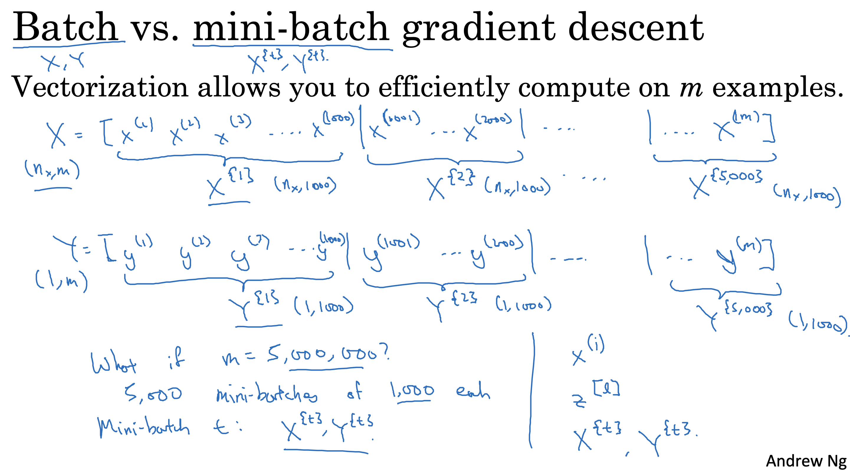
在单轮训练过程中,不再一次从计算整个训练数据,将整个训练数据分批进行训练,每批(epoch)训练的样本数称为batch size
batch size 最大等于整个训练样本数m时,相当于进行一次批量运算,就是标准的批量梯度下降算法,
需要计算完基于整个训练样本参数和损失函数,花费时间较长,然后才能进行梯度下降计算
1 | # (Batch) Gradient Descent: |
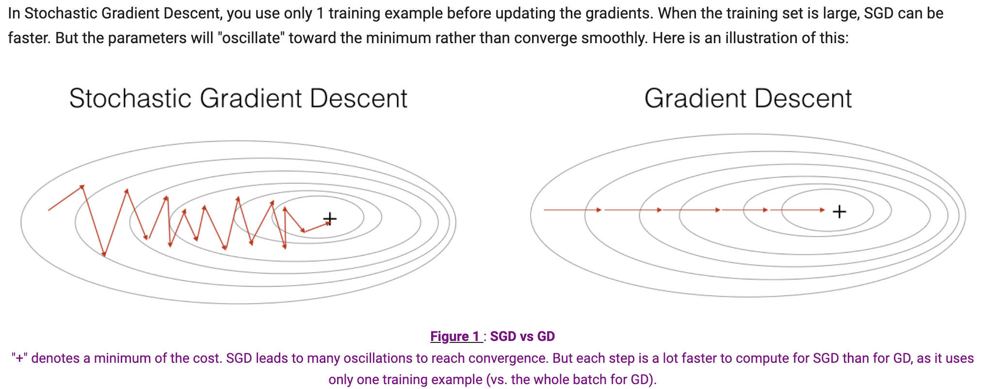
batch size 最小等于1时,就是一个批次处理一个数据, 速度快,但是没法利用向量加速梯度下降,也称为随机梯度下降算法Stochastic Gradient Descent:1
2
3
4
5
6
7
8
9
10
11
12
13
14# Stochastic Gradient Descent:
X = data_input
Y = labels
parameters = initialize_parameters(layers_dims)
for i in range(0, num_iterations):
for j in range(0, m):
# Forward propagation
a, caches = forward_propagation(X[:,j], parameters) # X[:,j] 从m列中,每次取一列,就是一个样本
# Compute cost
cost += compute_cost(a, Y[:,j])
# Backward propagation
grads = backward_propagation(a, caches, parameters)
# Update parameters.
parameters = update_parameters(parameters, grads)
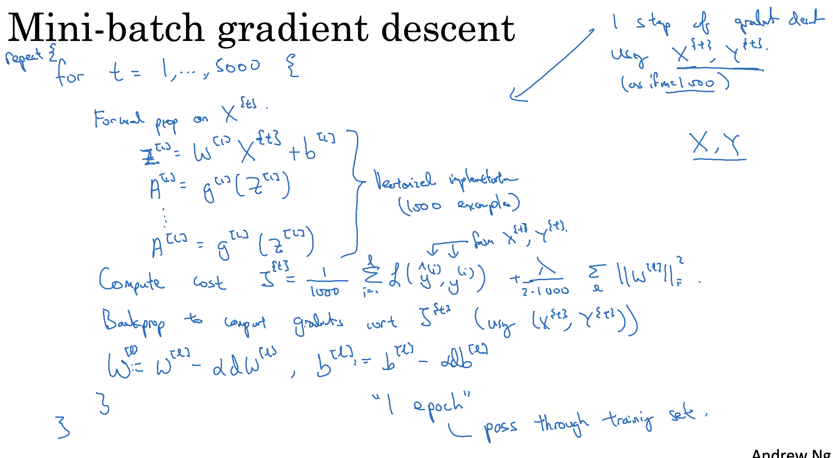
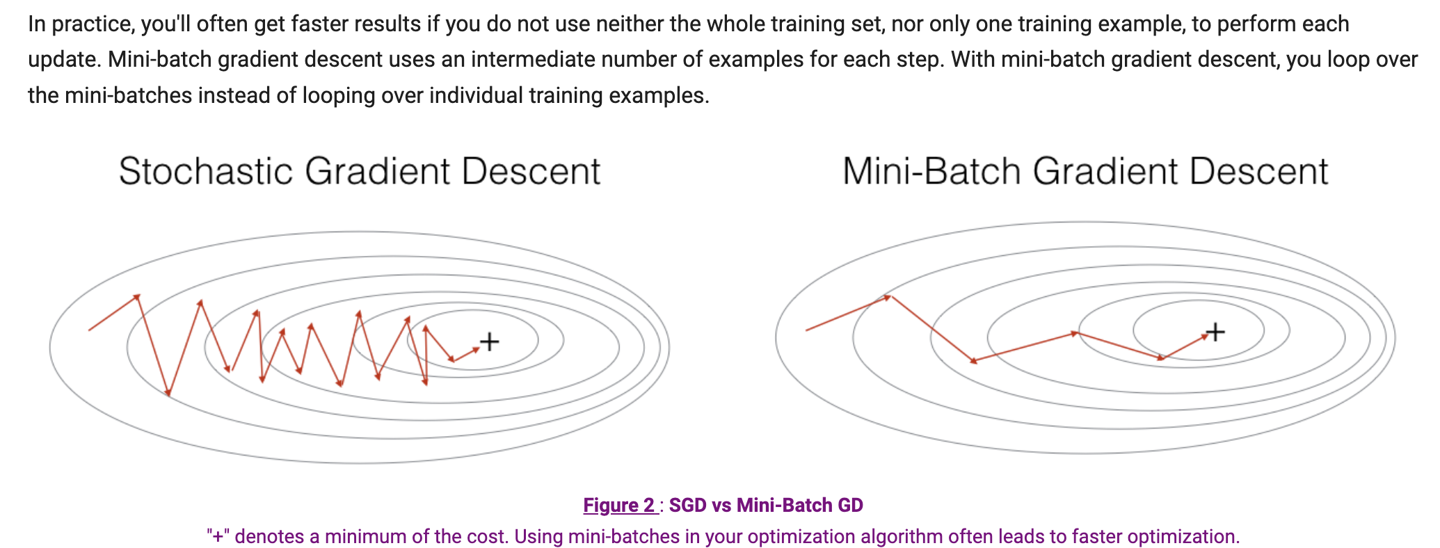
当batch size 介于1和m之间时,就是小批量梯度下降算法Mini-batch Gradient Descent
小批量梯度下降处理数据分两步,
一步是混洗数据,将数据集顺序打乱,但保证X(i) 和 Y(i)是一一对应的
第二步是将数据分成多个batch,每个batch包含batch size 个样本,需要注意如果m 不能整除batch size,最后一个batch 是不足batch size 个样本,需要单独处理
Shuffling and Partitioning are the two steps required to build mini-batches -
Powers of two are often chosen to be the mini-batch size, e.g., 16, 32, 64, 128.
1 | # GRADED FUNCTION: random_mini_batches |
迭代过程处理的数据集就是上面分批好的mini_batches
1 | mini_batches = random_mini_batches(X, Y, mini_batch_size = 64, seed = 0) |
The difference between gradient descent, mini-batch gradient descent and stochastic gradient descent is the number of examples you use to perform one update step. - You have to tune a learning rate hyperparameter 𝛼 . - With a well-turned mini-batch size, usually it outperforms either gradient descent or stochastic gradient descent (particularly when the training set is large).
momentum
指数加权平均
指数加权平均(Exponential Weighted Moving Average, EWMA)是一种用于平滑时间序列数据的技术。
它通过对数据点赋予不同的权重来计算平均值,较新的数据点权重较大,较旧的数据点权重较小。
这样可以更敏感地反映最新数据的变化,同时保留历史数据的趋势。
指数加权平均的计算公式如下:
St = β St-1 + (1-β) Xt
其中:
St是时间 t 时刻的指数加权平均值。
Xt是时间 t 时刻的实际数据值。
β 是平滑因子,取值范围在 0 到 1 之间。较大的 值使得 EWMA 对最新数据更敏感,较小的 值则使得 EWMA 更平滑。
St-1是时间 t-1 时刻的指数加权平均值。
解释
初始值:通常,初始的指数加权平均值 S0 可以设置为第一个数据点 X0 。
递归计算:每个新的数据点都会更新 EWMA,新的 EWMA 是当前数据点和前一个 EWMA 的加权和。
平滑因子 :决定了新数据点和历史数据对当前 EWMA 的影响程度。较大的 值会使得 EWMA 对新数据点变化更敏感,较小的 值会使得 EWMA 更平滑,受历史数据影响更大。
偏差修正
在计算 EWMA 时,初始值的选择对后续计算的影响较大。特别是在数据序列的初始阶段,
由于缺乏足够的历史数据,计算的平均值可能会偏离真实值。
因此,需要对初始阶段的计算结果进行修正,以减小这种偏差。
为了进行偏差修正,我们可以使用以下公式:
St^ = St / (1 - β^t)
其中:
St^是经过偏差修正的时间 t 时刻的指数加权平均值。
St是时间 t 时刻的未修正的指数加权平均值。
t是时间步数,从1 开始,它是β^t 是指β的 t 次方。
通过对初始值进行修正,我们可以使 EWMA 在初始阶段更接近真实值,从而减少偏差。
修正后的 EWMA 可以帮助我们更准确地反映数据的趋势和变化。
momentum
momentum 是一种优化算法,用于加速梯度下降过程。它通过引入动量(momentum)的概念来加速参数的更新。
在每次迭代中,momentum 会考虑上一次迭代的梯度方向,并根据动量的大小来调整当前的梯度方向。
这样可以在梯度下降的过程中,更加平滑地更新参数,从而加速收敛。
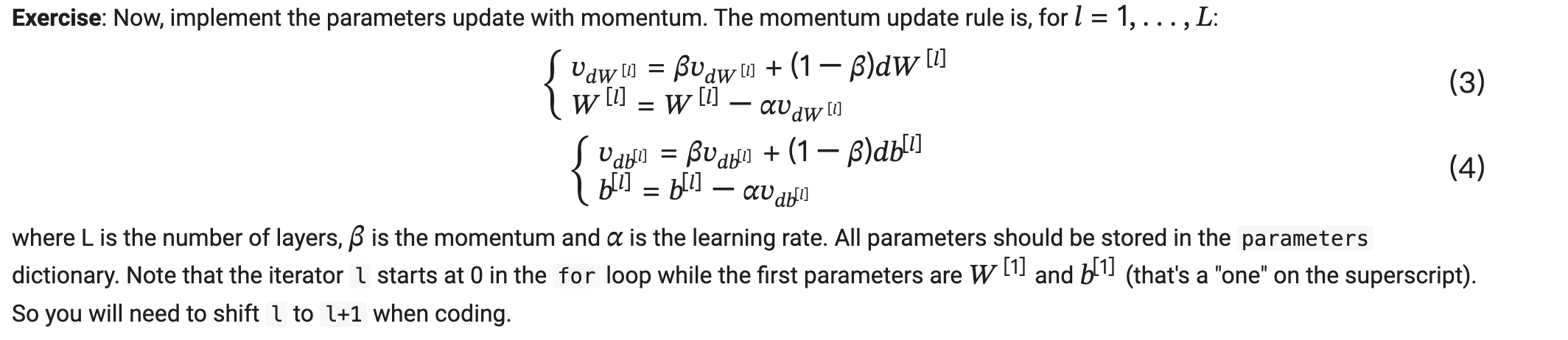
momentum 的计算公式如下:
VdW = β VdW + (1 - β) dW
Vdb = β Vdb + (1 - β) db
W = W - α VdW
b = b - α Vdb
其中:
VdW是权重参数W的动量。
Vdb是偏置参数b的动量。
dW是权重参数W的梯度。
db是偏置参数b的梯度。
α是学习率。
β是动量因子,通常取值在0.9到0.99之间。
由于小批量梯度下降所采用的路径将“振荡”至收敛,利用momentum可以减少这些振荡。
(将VdW,带入W更新式子计算,会发现 W 下降的比之前要慢一些,负负得正,会加回来-β VdW + β dW)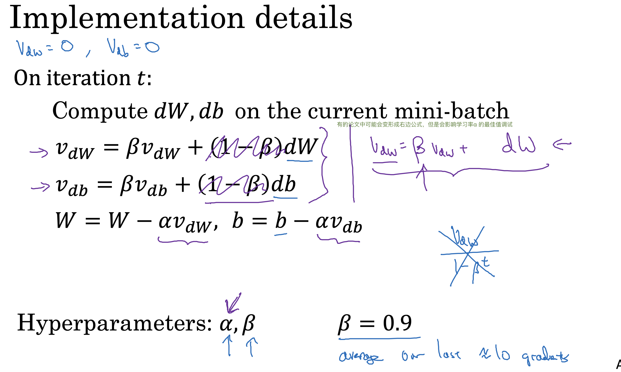
1
2
3
4
5
6
7
8
9
10
11
12
13
14
15
16
17
18
19
20
21
22
23
24
25
26
27# GRADED FUNCTION: initialize_velocity
def initialize_velocity(parameters):
"""
Initializes the velocity as a python dictionary with:
- keys: "dW1", "db1", ..., "dWL", "dbL"
- values: numpy arrays of zeros of the same shape as the corresponding gradients/parameters.
Arguments:
parameters -- python dictionary containing your parameters.
parameters['W' + str(l)] = Wl
parameters['b' + str(l)] = bl
Returns:
v -- python dictionary containing the current velocity.
v['dW' + str(l)] = velocity of dWl
v['db' + str(l)] = velocity of dbl
"""
L = len(parameters) // 2 # number of layers in the neural networks
v = {}
# Initialize velocity
for l in range(L):
v["dW" + str(l+1)] = np.zeros_like(parameters["W" + str(l+1)])
v["db" + str(l+1)] = np.zeros_like(parameters["b" + str(l+1)])
return v
1 |
|
Note that:
The velocity is initialized with zeros. So the algorithm will take a few iterations to “build up” velocity and start to take bigger steps.
If 𝛽=0 , then this just becomes standard gradient descent without momentum.
How do you choose 𝛽 ?
The larger the momentum 𝛽 is, the smoother the update because the more we take the past gradients into account. But if 𝛽 is too big, it could also smooth out the updates too much.
Common values for 𝛽 range from 0.8 to 0.999. If you don’t feel inclined to tune this, 𝛽=0.9 is often a reasonable default.
Tuning the optimal 𝛽 for your model might need trying several values to see what works best in term of reducing the value of the cost function 𝐽 .
Momentum takes past gradients into account to smooth out the steps of gradient descent. It can be applied with batch gradient descent, mini-batch gradient descent or stochastic gradient descent. - You have to tune a momentum hyperparameter 𝛽 and a learning rate 𝛼 .
Adam
RMSprop
Root Mean Square Propagation
类似指数加权平均,在更改更新梯度的逻辑,不再直接减去学习率乘以梯度,而是减去学习率乘以优化处理后的梯度值,详见如下公式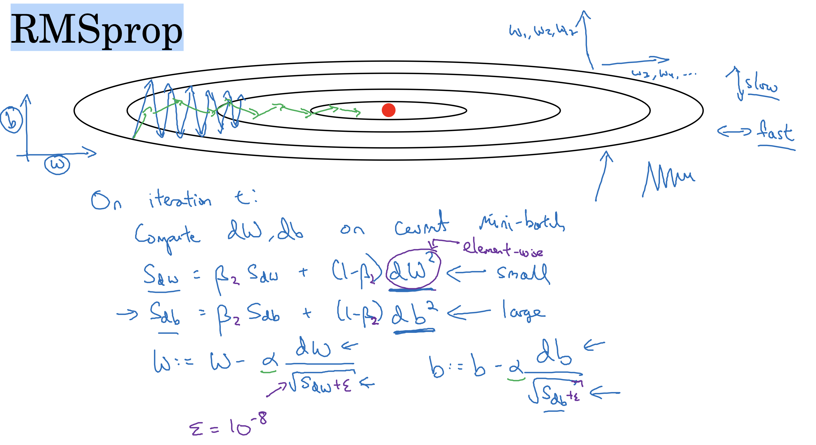
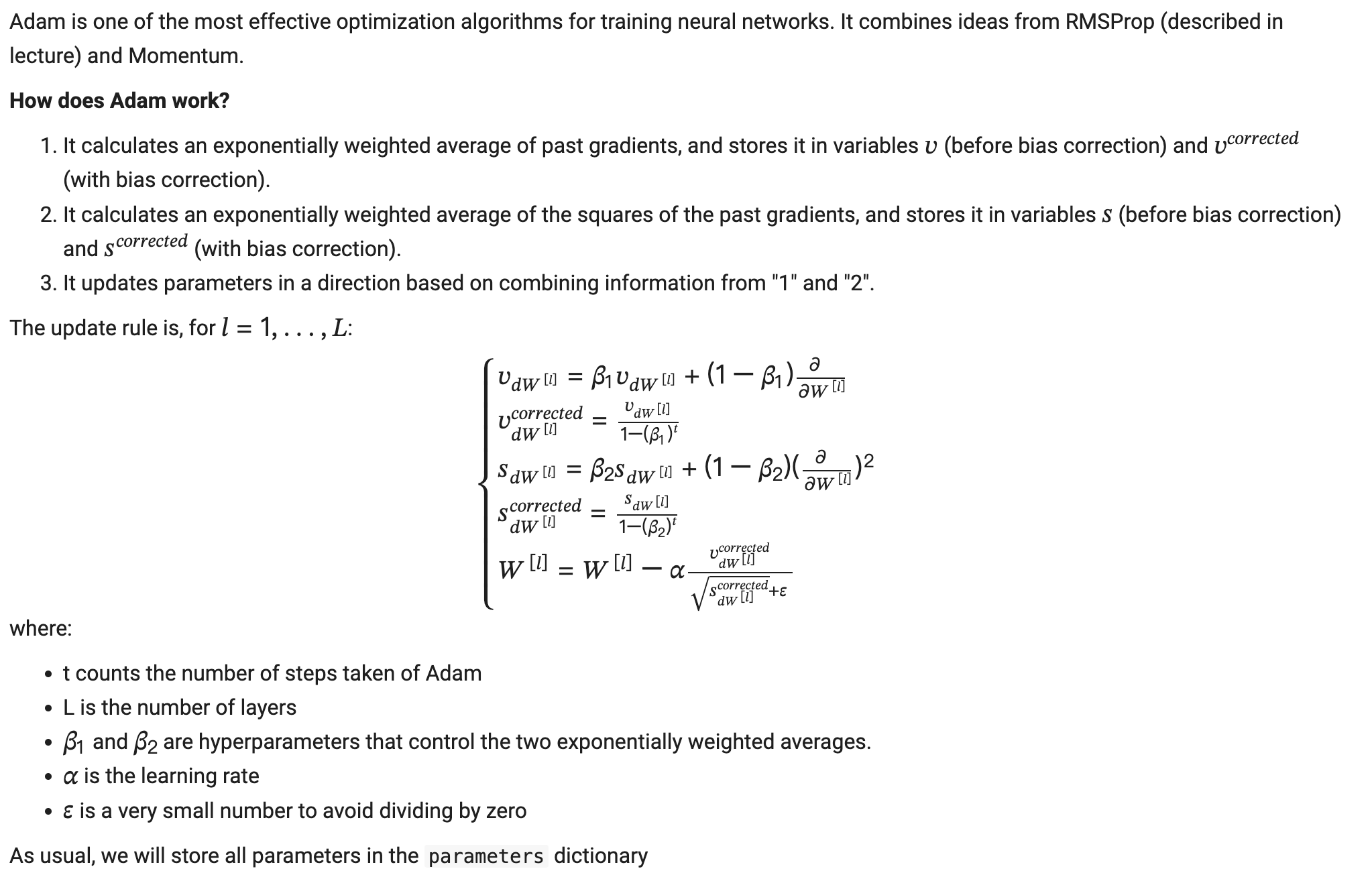
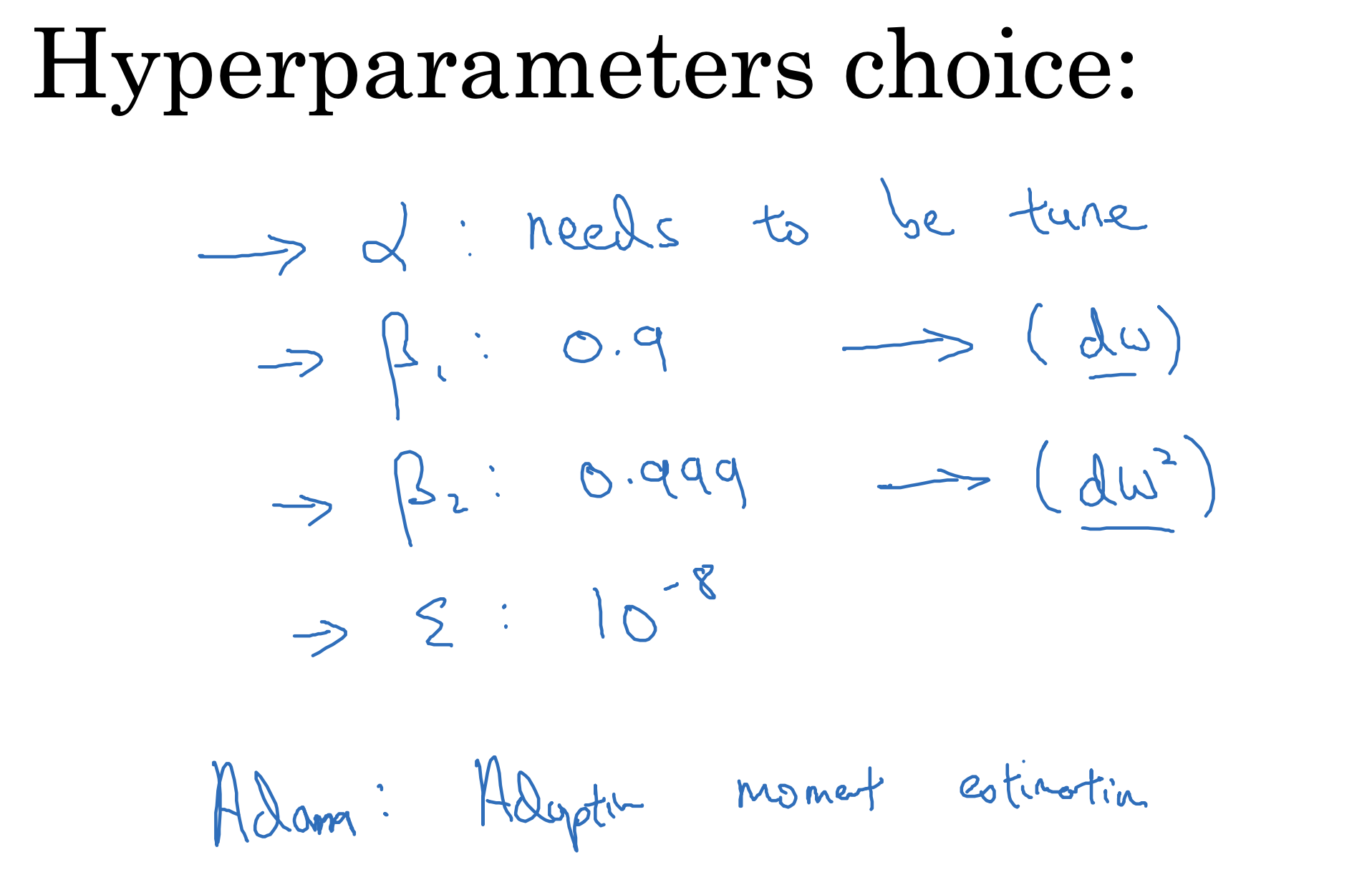
Adam 优化算法
结合指数平均和RMSprop两种算法更新梯度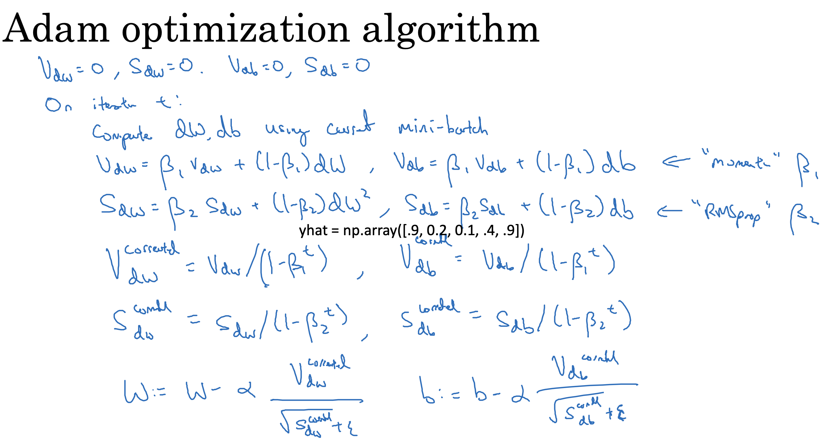
1
2
3
4
5
6
7
8
9
10
11
12
13
14
15
16
17
18
19
20
21
22
23
24
25
26
27
28
29
30
31
32
33
34
35
36
37
38
39
40
41
42
43
44
45
46
47
48
49
50
51
52
53
54
55
56
57
58
59
60
61
62
63
64
65
66
67
68
69
70
71
72
73
74
75
76
77
78
79
80
81
82
83
84
85
86
87
88
89
90# GRADED FUNCTION: initialize_adam
def initialize_adam(parameters) :
"""
Initializes v and s as two python dictionaries with:
- keys: "dW1", "db1", ..., "dWL", "dbL"
- values: numpy arrays of zeros of the same shape as the corresponding gradients/parameters.
Arguments:
parameters -- python dictionary containing your parameters.
parameters["W" + str(l)] = Wl
parameters["b" + str(l)] = bl
Returns:
v -- python dictionary that will contain the exponentially weighted average of the gradient.
v["dW" + str(l)] = ...
v["db" + str(l)] = ...
s -- python dictionary that will contain the exponentially weighted average of the squared gradient.
s["dW" + str(l)] = ...
s["db" + str(l)] = ...
"""
L = len(parameters) // 2 # number of layers in the neural networks
v = {}
s = {}
# Initialize v, s. Input: "parameters". Outputs: "v, s".
for l in range(L):
v["dW" + str(l+1)] = np.zeros_like(parameters["W" + str(l+1)])
v["db" + str(l+1)] = np.zeros_like(parameters["b" + str(l+1)])
s["dW" + str(l+1)] = np.zeros_like(parameters["W" + str(l+1)])
s["db" + str(l+1)] = np.zeros_like(parameters["b" + str(l+1)])
return v, s
# GRADED FUNCTION: update_parameters_with_adam
def update_parameters_with_adam(parameters, grads, v, s, t, learning_rate = 0.01,
beta1 = 0.9, beta2 = 0.999, epsilon = 1e-8):
"""
Update parameters using Adam
Arguments:
parameters -- python dictionary containing your parameters:
parameters['W' + str(l)] = Wl
parameters['b' + str(l)] = bl
grads -- python dictionary containing your gradients for each parameters:
grads['dW' + str(l)] = dWl
grads['db' + str(l)] = dbl
v -- Adam variable, moving average of the first gradient, python dictionary
s -- Adam variable, moving average of the squared gradient, python dictionary
learning_rate -- the learning rate, scalar.
beta1 -- Exponential decay hyperparameter for the first moment estimates
beta2 -- Exponential decay hyperparameter for the second moment estimates
epsilon -- hyperparameter preventing division by zero in Adam updates
Returns:
parameters -- python dictionary containing your updated parameters
v -- Adam variable, moving average of the first gradient, python dictionary
s -- Adam variable, moving average of the squared gradient, python dictionary
"""
L = len(parameters) // 2 # number of layers in the neural networks
v_corrected = {} # Initializing first moment estimate, python dictionary
s_corrected = {} # Initializing second moment estimate, python dictionary
# Perform Adam update on all parameters
for l in range(L):
# Moving average of the gradients. Inputs: "v, grads, beta1". Output: "v".
v["dW" + str(l+1)] = beta1 * v["dW" + str(l+1)] + (1 - beta1) * grads["dW" + str(l+1)]
v["db" + str(l+1)] = beta1 * v["db" + str(l+1)] + (1 - beta1) * grads["db" + str(l+1)]
# Compute bias-corrected first moment estimate. Inputs: "v, beta1, t". Output: "v_corrected".
v_corrected["dW" + str(l+1)] = v["dW" + str(l+1)] / (1 - beta1 ** t)
v_corrected["db" + str(l+1)] = v["db" + str(l+1)] / (1 - beta1 ** t)
# Moving average of the squared gradients. Inputs: "s, grads, beta2". Output: "s".
s["dW" + str(l+1)] = beta2 * s["dW" + str(l+1)] + (1 - beta2) * grads["dW" + str(l+1)] ** 2
s["db" + str(l+1)] = beta2 * s["db" + str(l+1)] + (1 - beta2) * grads["db" + str(l+1)] ** 2
# Compute bias-corrected second raw moment estimate. Inputs: "s, beta2, t". Output: "s_corrected".
s_corrected["dW" + str(l+1)] = s["dW" + str(l+1)] / (1 - beta2 ** t)
s_corrected["db" + str(l+1)] = s["db" + str(l+1)] / (1 - beta2 ** t)
# Update parameters. Inputs: "parameters, learning_rate, v_corrected, s_corrected, epsilon". Output: "parameters".
parameters["W" + str(l+1)] -= learning_rate * v_corrected["dW" + str(l+1)] / (np.sqrt(s_corrected["dW" + str(l+1)]) + epsilon)
parameters["b" + str(l+1)] -= learning_rate * v_corrected["db" + str(l+1)] / (np.sqrt(s_corrected["db" + str(l+1)]) + epsilon)
return parameters, v, s
实验
小结
Momentum usually helps, but given the small learning rate and the simplistic dataset, its impact is almost negligeable. Also, the huge oscillations you see in the cost come from the fact that some minibatches are more difficult thans others for the optimization algorithm.
Adam on the other hand, clearly outperforms mini-batch gradient descent and Momentum. If you run the model for more epochs on this simple dataset, all three methods will lead to very good results. However, you’ve seen that Adam converges a lot faster.
实验效果Adam算法速度快,准确率高
Some advantages of Adam include:
Relatively low memory requirements (though higher than gradient descent and gradient descent with momentum)
Usually works well even with little tuning of hyperparameters (except 𝛼 )
学习率衰减
在小批量梯度下降计算过程中,随着计算批次后移,逐渐减小学习率的值,可以降低梯度震荡幅度,加速收敛速度
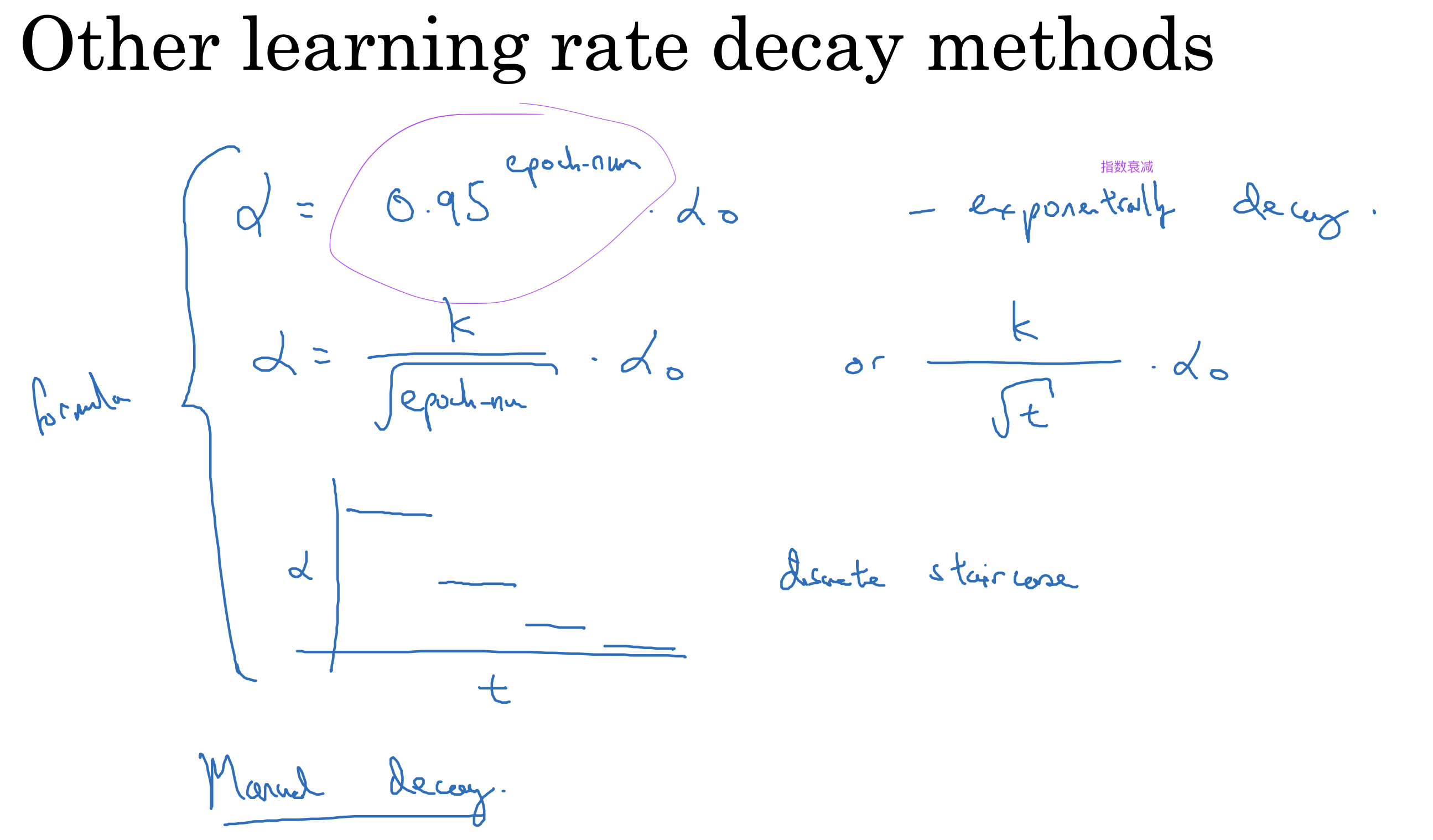
一些学习率衰减算法如下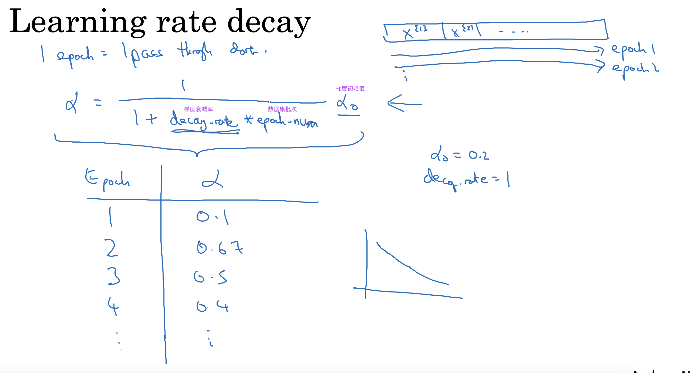
两个经验法则
Unlikely to get stuck in a bad local optima 一般不存在局部最优解,损失函数与参数关系往往成马鞍装
Plateaus can make learning slow 平缓的地方往往会造成学习速度下降,需要花费更多时间找到更优解